
|
|
|
 הצגת notebook ב-GitHub הצגת notebook ב-GitHub
|
סקירה כללית
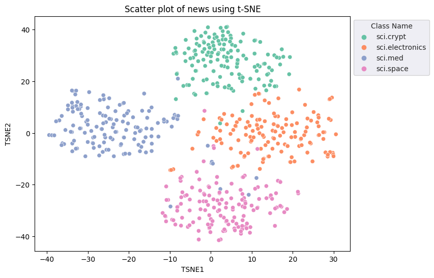
במדריך הזה נדגים איך להשתמש בהטמעות מ-Gemini API כדי לזהות חריגים יוצאי דופן במערך הנתונים. תוכלו להמחיש קבוצת משנה של 20 מערך הנתונים של Newsgroup באמצעות t-SNE ולזהות חריגים מחוץ לרדיוס מסוים של הנקודה המרכזית של כל אשכול קטגורי.
למידע נוסף על תחילת העבודה עם הטמעות שנוצרו מ-Gemini API, תוכלו לעיין במדריך למתחילים בנושא Python.
דרישות מוקדמות
אפשר להפעיל את המדריך למתחילים הזה ב-Google Colab.
כדי להשלים את המדריך למתחילים הזה בסביבת הפיתוח שלכם, צריך לוודא שהסביבה שלכם עומדת בדרישות הבאות:
- Python 3.9 ואילך
- התקנה של
jupyterכדי להריץ את ה-notebook.
הגדרה
קודם כול, מורידים ומתקינים את ספריית Python של Gemini API.
pip install -U -q google.generativeai
import re
import tqdm
import numpy as np
import pandas as pd
import matplotlib.pyplot as plt
import seaborn as sns

import google.generativeai as genai

# Used to securely store your API key
from google.colab import userdata

from sklearn.datasets import fetch_20newsgroups
from sklearn.manifold import TSNE
קבלת מפתח API
כדי להשתמש ב-Gemini API, קודם צריך לקבל מפתח API. אם עדיין אין לכם מפתח, אתם יכולים ליצור מפתח בלחיצה אחת ב-Google AI Studio.
ב-Colab, מוסיפים את המפתח למנהל הסודות מתחת לכיתוב '🔑' בחלונית הימנית. נותנים למכשיר את השם API_KEY.
אחרי שמקבלים את מפתח ה-API, מעבירים אותו ל-SDK. תוכל לעשות זאת בשתי דרכים:
- מכניסים את המפתח למשתנה הסביבה
GOOGLE_API_KEY(ערכת ה-SDK תאסוף אותו משם באופן אוטומטי). - צריך להעביר את המפתח אל
genai.configure(api_key=...)
genai.configure(api_key=GOOGLE_API_KEY)
for m in genai.list_models():
  if 'embedContent' in m.supported_generation_methods:
    print(m.name)
models/embedding-001
models/embedding-001
הכנת מערך הנתונים
מערך נתוני הטקסט של 20 קבוצות חדשות מכיל 18,000 פוסטים של קבוצות חדשות ב-20 נושאים, המחולקים לערכות של אימון ובדיקה. החלוקה בין מערכי הנתונים לאימון ולמבחן מבוססת על הודעות שפורסמו לפני ואחרי תאריך מסוים. המדריך הזה משתמש בקבוצת המשנה לאימון.
newsgroups_train = fetch_20newsgroups(subset='train')

# View list of class names for dataset
newsgroups_train.target_names
['alt.atheism',
 'comp.graphics',
 'comp.os.ms-windows.misc',
 'comp.sys.ibm.pc.hardware',
 'comp.sys.mac.hardware',
 'comp.windows.x',
 'misc.forsale',
 'rec.autos',
 'rec.motorcycles',
 'rec.sport.baseball',
 'rec.sport.hockey',
 'sci.crypt',
 'sci.electronics',
 'sci.med',
 'sci.space',
 'soc.religion.christian',
 'talk.politics.guns',
 'talk.politics.mideast',
 'talk.politics.misc',
 'talk.religion.misc']
זאת הדוגמה הראשונה בערכת האימון.
idx = newsgroups_train.data[0].index('Lines')
print(newsgroups_train.data[0][idx:])
Lines: 15

 I was wondering if anyone out there could enlighten me on this car I saw
the other day. It was a 2-door sports car, looked to be from the late 60s/
early 70s. It was called a Bricklin. The doors were really small. In addition,
the front bumper was separate from the rest of the body. This is
all I know. If anyone can tellme a model name, engine specs, years
of production, where this car is made, history, or whatever info you
have on this funky looking car, please e-mail.

Thanks,

- IL
   ---- brought to you by your neighborhood Lerxst ----
# Apply functions to remove names, emails, and extraneous words from data points in newsgroups.data
newsgroups_train.data = [re.sub(r'[\w\.-]+@[\w\.-]+', '', d) for d in newsgroups_train.data] # Remove email
newsgroups_train.data = [re.sub(r"\([^()]*\)", "", d) for d in newsgroups_train.data] # Remove names
newsgroups_train.data = [d.replace("From: ", "") for d in newsgroups_train.data] # Remove "From: "
newsgroups_train.data = [d.replace("\nSubject: ", "") for d in newsgroups_train.data] # Remove "\nSubject: "

# Cut off each text entry after 5,000 characters
newsgroups_train.data = [d[0:5000] if len(d) > 5000 else d for d in newsgroups_train.data]
# Put training points into a dataframe
df_train = pd.DataFrame(newsgroups_train.data, columns=['Text'])
df_train['Label'] = newsgroups_train.target
# Match label to target name index
df_train['Class Name'] = df_train['Label'].map(newsgroups_train.target_names.__getitem__)

df_train
בשלב הבא, תוכלו לדגום חלק מהנתונים על ידי איסוף של 150 נקודות במערך הנתונים לאימון, ובחירה של מספר קטגוריות. המדריך הזה משתמש בקטגוריות המדעיות.
# Take a sample of each label category from df_train
SAMPLE_SIZE = 150
df_train = (df_train.groupby('Label', as_index = False)
                    .apply(lambda x: x.sample(SAMPLE_SIZE))
                    .reset_index(drop=True))

# Choose categories about science
df_train = df_train[df_train['Class Name'].str.contains('sci')]

# Reset the index
df_train = df_train.reset_index()
df_train
df_train['Class Name'].value_counts()
sci.crypt          150
sci.electronics    150
sci.med            150
sci.space          150
Name: Class Name, dtype: int64
יצירת הטמעות
בקטע הזה נסביר איך ליצור הטמעות לטקסטים השונים ב-dataframe באמצעות הטמעות מ-Gemini API.
שינויים ב-API של הטמעות עם מודל הטמעת מודל-001
למודל ההטמעות החדש, embed-001, יש פרמטר חדש של סוג משימה והכותרת האופציונלית (רלוונטי רק ל-task_type=RETRIEVAL_DOCUMENT).
הפרמטרים החדשים האלה רלוונטיים רק למודלים החדשים ביותר של הטמעות.סוגי המשימות הם:
| סוג המשימה | תיאור |
|---|---|
| RETRIEVAL_QUERY | מציינת שהטקסט הנתון הוא שאילתה בהגדרת חיפוש/אחזור. |
| RETRIEVAL_DOCUMENT | מציינת שהטקסט הנתון הוא מסמך בהגדרת חיפוש/אחזור. |
| SEMANTIC_SIMILARITY | מציינת שהטקסט הנתון ישמש לדמיון סמנטי (STS). |
| סיווג | מציינת שההטמעות ישמשו לסיווג. |
| אשכול | מציינת שההטמעות ישמשו לקיבוץ לאשכולות. |
from tqdm.auto import tqdm
tqdm.pandas()

from google.api_core import retry

def make_embed_text_fn(model):

  @retry.Retry(timeout=300.0)
  def embed_fn(text: str) -> list[float]:
    # Set the task_type to CLUSTERING.
    embedding = genai.embed_content(model=model,
                                    content=text,
                                    task_type="clustering")['embedding']
    return np.array(embedding)

  return embed_fn

def create_embeddings(df):
  model = 'models/embedding-001'
  df['Embeddings'] = df['Text'].progress_apply(make_embed_text_fn(model))
  return df

df_train = create_embeddings(df_train)
df_train.drop('index', axis=1, inplace=True)
0%| | 0/600 [00:00<?, ?it/s]
צמצום ממדים
הממד של וקטור הטמעת המסמך הוא 768. כדי להמחיש את אופן קיבוץ המסמכים המוטמעים יחד, צריך להשתמש בתכונה 'הפחתת מידות', מכיוון שניתן להמחיש את ההטמעות רק בסביבה דו-ממדית או בתלת-ממד. מסמכים דומים לפי הקשר צריכים להיות קרובים יותר זה לזה במרחב, בניגוד למסמכים שאינם דומים זה לזה.
len(df_train['Embeddings'][0])
768
# Convert df_train['Embeddings'] Pandas series to a np.array of float32
X = np.array(df_train['Embeddings'].to_list(), dtype=np.float32)
X.shape
(600, 768)
תפעילו את הגישה של הטמעה של שכנות סטוכסטיות ב-t (t-SNE) כדי לבצע הפחתת ממדים. השיטה הזו מצמצמת את מספר המאפיינים תוך שימור אשכולות (נקודות שקרובות זו לזו נשארות קרובות זו לזו). על הנתונים המקוריים, המודל מנסה ליצור התפלגות שעליה נקודות נתונים אחרות הן "שכנות" (למשל, אם יש להם משמעות דומה). לאחר מכן, המערכת מבצעת אופטימיזציה של פונקציית יעד כדי לשמור על התפלגות דומה בתצוגה החזותית.
tsne = TSNE(random_state=0, n_iter=1000)
tsne_results = tsne.fit_transform(X)
df_tsne = pd.DataFrame(tsne_results, columns=['TSNE1', 'TSNE2'])
df_tsne['Class Name'] = df_train['Class Name'] # Add labels column from df_train to df_tsne
df_tsne
fig, ax = plt.subplots(figsize=(8,6)) # Set figsize
sns.set_style('darkgrid', {"grid.color": ".6", "grid.linestyle": ":"})
sns.scatterplot(data=df_tsne, x='TSNE1', y='TSNE2', hue='Class Name', palette='Set2')
sns.move_legend(ax, "upper left", bbox_to_anchor=(1, 1))
plt.title('Scatter plot of news using t-SNE')
plt.xlabel('TSNE1')
plt.ylabel('TSNE2');
זיהוי חריג חשוד טעות
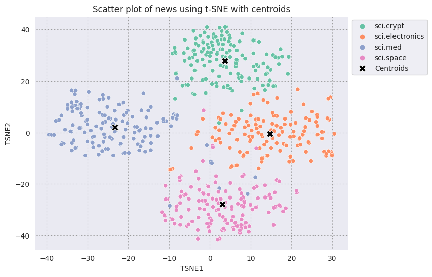
כדי לקבוע אילו נקודות הן חריגות, אתם צריכים לקבוע אילו נקודות הן חריגות וחריגות. בתור התחלה, מצאו את מרכז האשכול, או המיקום שמייצג את מרכז האשכול, והשתמשו במרחק כדי לקבוע את הנקודות חריגות.
קודם כול צריך לקבל את המרכז של כל קטגוריה.
def get_centroids(df_tsne):
  # Get the centroid of each cluster
  centroids = df_tsne.groupby('Class Name').mean()
  return centroids

centroids = get_centroids(df_tsne)
centroids
def get_embedding_centroids(df):
  emb_centroids = dict()
  grouped = df.groupby('Class Name')
  for c in grouped.groups:
    sub_df = grouped.get_group(c)
    # Get the centroid value of dimension 768
    emb_centroids[c] = np.mean(sub_df['Embeddings'], axis=0)

  return emb_centroids
emb_c = get_embedding_centroids(df_train)
ציירו כל נקודת המרכז שמצאתם מול שאר הנקודות.
# Plot the centroids against the cluster
fig, ax = plt.subplots(figsize=(8,6)) # Set figsize
sns.set_style('darkgrid', {"grid.color": ".6", "grid.linestyle": ":"})
sns.scatterplot(data=df_tsne, x='TSNE1', y='TSNE2', hue='Class Name', palette='Set2');
sns.scatterplot(data=centroids, x='TSNE1', y='TSNE2', color="black", marker='X', s=100, label='Centroids')
sns.move_legend(ax, "upper left", bbox_to_anchor=(1, 1))
plt.title('Scatter plot of news using t-SNE with centroids')
plt.xlabel('TSNE1')
plt.ylabel('TSNE2');
בוחרים רדיוס. כל דבר מעבר לתחום זה נחשב למרכז של קטגוריה זו, שנחשב לחריג חשוד טעות.
def calculate_euclidean_distance(p1, p2):
  return np.sqrt(np.sum(np.square(p1 - p2)))

def detect_outlier(df, emb_centroids, radius):
  for idx, row in df.iterrows():
    class_name = row['Class Name'] # Get class name of row
    # Compare centroid distances
    dist = calculate_euclidean_distance(row['Embeddings'],
                                        emb_centroids[class_name])
    df.at[idx, 'Outlier'] = dist > radius

  return len(df[df['Outlier'] == True])
range_ = np.arange(0.3, 0.75, 0.02).round(decimals=2).tolist()
num_outliers = []
for i in range_:
  num_outliers.append(detect_outlier(df_train, emb_c, i))
# Plot range_ and num_outliers
fig = plt.figure(figsize = (14, 8))
plt.rcParams.update({'font.size': 12})
plt.bar(list(map(str, range_)), num_outliers)
plt.title("Number of outliers vs. distance of points from centroid")
plt.xlabel("Distance")
plt.ylabel("Number of outliers")
for i in range(len(range_)):
  plt.text(i, num_outliers[i], num_outliers[i], ha = 'center')

plt.show()
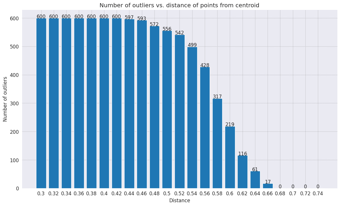
בהתאם לרגישות הרצויה של גלאי האנומליות, ניתן לבחור באיזה רדיוס להשתמש. כרגע נעשה שימוש בערך 0.62, אבל אפשר לשנות את הערך הזה.
# View the points that are outliers
RADIUS = 0.62
detect_outlier(df_train, emb_c, RADIUS)
df_outliers = df_train[df_train['Outlier'] == True]
df_outliers.head()
# Use the index to map the outlier points back to the projected TSNE points
outliers_projected = df_tsne.loc[df_outliers['Outlier'].index]
ציירו את נקודות החריגות ומסומנות בצבע אדום שקוף.
fig, ax = plt.subplots(figsize=(8,6)) # Set figsize
plt.rcParams.update({'font.size': 10})
sns.set_style('darkgrid', {"grid.color": ".6", "grid.linestyle": ":"})
sns.scatterplot(data=df_tsne, x='TSNE1', y='TSNE2', hue='Class Name', palette='Set2');
sns.scatterplot(data=centroids, x='TSNE1', y='TSNE2', color="black", marker='X', s=100, label='Centroids')
# Draw a red circle around the outliers
sns.scatterplot(data=outliers_projected, x='TSNE1', y='TSNE2', color='red', marker='o', alpha=0.5, s=90, label='Outliers')
sns.move_legend(ax, "upper left", bbox_to_anchor=(1, 1))
plt.title('Scatter plot of news with outliers projected with t-SNE')
plt.xlabel('TSNE1')
plt.ylabel('TSNE2');
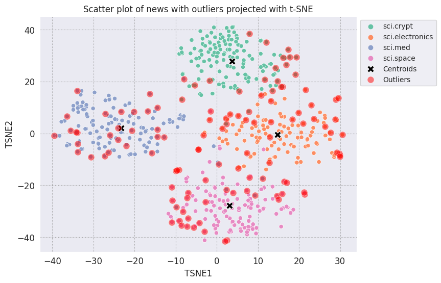
ניתן להשתמש בערכי האינדקס של פלטפורמות הנתונים כדי להדפיס מספר דוגמאות לערכי חריגים שעשויים להיראות בכל קטגוריה. כאן מודפסת הנקודה הראשונה על הגרף מכל קטגוריה. עיינו בנקודות נוספות בכל קטגוריה כדי לראות נתונים שנחשבים כחריגים או חריגות.
sci_crypt_outliers = df_outliers[df_outliers['Class Name'] == 'sci.crypt']
print(sci_crypt_outliers['Text'].iloc[0])
Re: Source of random bits on a Unix workstation
Lines: 44
Nntp-Posting-Host: sandstorm

>>For your application, what you can do is to encrypt the real-time clock
>>value with a secret key.

Well, almost.... If I only had to solve the problem for myself, and were
willing to have to type in a second password  whenever I
logged in, it could work. However, I'm trying to create a solution that
anyone can use, and which, once installed, is just as effortless to start up
as the non-solution of just using xhost to control access. I've got
religeous problems with storing secret keys on multiuser computers.

>For a good discussion of cryptographically "good" random number
>generators, check out the draft-ietf-security-randomness-00.txt
>Internet Draft, available at your local friendly internet drafts
>repository.

Thanks for the pointer! It was good reading, and I liked the idea of using
several unrelated sources with a strong mixing function. However, unless I
missed something, the only source they suggested
that seems available, and unguessable by an intruder, when a Unix is
fresh-booted, is I/O buffers related to network traffic. I believe my
solution basically uses that strategy, without requiring me to reach into
the kernel.

>A reasonably source of randomness is the output of a cryptographic
>hash function , when fed with a large amount of
>more-or-less random data. For example, running MD5 on /dev/mem is a
>slow, but random enough, source of random bits; there are bound to be
>128 bits of entropy in the tens  of megabytes of data in
>a modern workstation's memory, as a fair amount of them are system
>timers, i/o buffers, etc.

I heard about this solution, and it sounded good. Then I heard that folks
were experiencing times of 30-60 seconds to run this, on
reasonably-configured workstations. I'm not willing to add that much delay
to someone's login process. My approach  takes
a second or two to run. I'm considering writing the be-all and end-all of
solutions, that launches the MD5, and simultaneously tries to suck bits off
the net, and if the net should be sitting __SO__ idle that it can't get 10K
after compression before MD5 finishes, use the MD5. This way I could have
guaranteed good bits, and a deterministic upper bound on login time, and
still have the common case of login take only a couple of extra seconds.

-Bennett
sci_elec_outliers = df_outliers[df_outliers['Class Name'] == 'sci.electronics']
print(sci_elec_outliers['Text'].iloc[0])
Re: Laser vs Bubblejet?
Reply-To:
Distribution: world
X-Mailer: cppnews \\(Revision: 1.20 \\)
Organization: null
Lines: 53

Here is a different viewpoint.

> FYI:  The actual horizontal dot placement resoution of an HP
> deskjet is 1/600th inch.  The electronics and dynamics of the ink
> cartridge, however, limit you to generating dots at 300 per inch.
> On almost any paper, the ink wicks more than 1/300th inch anyway.
>
> The method of depositing and fusing toner of a laster printer
> results in much less spread than ink drop technology.

In practice there is little difference in quality but more care is needed
with inkjet because smudges etc. can happen.

> It doesn't take much investigation to see that the mechanical and
> electronic complement of a laser printer is more complex than
> inexpensive ink jet printers.  Recall also that laser printers
> offer a much higher throughput:  10 ppm for a laser versus about 1
> ppm for an ink jet printer.

A cheap laser printer does not manage that sort of throughput and on top of
that how long does the _first_ sheet take to print? Inkjets are faster than
you say and in both cases the computer often has trouble keeping up with the
printer.

A sage said to me: "Do you want one copy or lots of copies?", "One",
"Inkjet".

> Something else to think about is the cost of consumables over the
> life of the printer.  A 3000 page yield toner cartridge is about
> $US 75-80 at discount while HP high capacity
> cartridges are about $US 22 at discount.  It could be that over the
> life cycle of the printer that consumables for laser printers are
> less than ink jet printers.  It is getting progressively closer
> between the two technologies.  Laser printers are usually desinged
> for higher duty cycles in pages per month and longer product
> replacement cycles.

Paper cost is the same and both can use refills. Long term the laserprinter
will need some expensive replacement parts  and on top of that
are the amortisation costs which favour the lowest purchase cost printer.

HP inkjets understand PCL so in many cases a laserjet driver will work if the
software package has no inkjet driver.

There is one wild difference between the two printers: a laserprinter is a
page printer whilst an inkjet is a line printer. This means that a
laserprinter can rotate graphic images whilst an inkjet cannot. Few drivers
actually use this facility.


  TC.
    E-mail:  or
sci_med_outliers = df_outliers[df_outliers['Class Name'] == 'sci.med']
print(sci_med_outliers['Text'].iloc[0])
Re: THE BACK MACHINE - Update
Organization: University of Nebraska--Lincoln
Lines: 15
Distribution: na
NNTP-Posting-Host: unlinfo.unl.edu

   I have a BACK MACHINE and have had one since January.  While I have not
found it to be a panacea for my back pain, I think it has helped somewhat.
It MAINLY acts to stretch muscles in the back and prevent spasms associated
with pain.  I am taking less pain medication than I was previously.
   The folks at BACK TECHNOLOGIES are VERY reluctant to honor their return
policy.  They extended my "warranty" period rather than allow me to return
the machine when, after the first month or so, I was not thrilled with it.
They encouraged me to continue to use it, abeit less vigourously.
   Like I said, I can't say it is a cure-all, but it keeps me stretched out
and I am in less pain.
--
***********************************************************************
Dale M. Webb, DVM, PhD           *  97% of the body is water.  The
Veterinary Diagnostic Center     *  other 3% keeps you from drowning.
University of Nebraska, Lincoln  *
sci_space_outliers = df_outliers[df_outliers['Class Name'] == 'sci.space']
print(sci_space_outliers['Text'].iloc[0])
MACH 25 landing site bases?
Article-I.D.: aurora.1993Apr5.193829.1
Organization: University of Alaska Fairbanks
Lines: 7
Nntp-Posting-Host: acad3.alaska.edu

The supersonic booms hear a few months ago over I belive San Fran, heading east
of what I heard, some new super speed Mach 25 aircraft?? What military based
int he direction of flight are there that could handle a Mach 25aircraft on its
landing decent?? Odd question??

==
Michael Adams,  -- I'm not high, just jacked
השלבים הבאים
יצרת עכשיו מזהה אנומליות באמצעות הטמעות! נסו להשתמש בנתונים טקסטואליים משלכם כדי להציג אותם כהטמעות, ולבחור גבולות כך שתוכלו לזהות חריגים. אפשר לבצע הפחתת מידות כדי להשלים את שלב התצוגה החזותית. שימו לב ש-t-SNE טוב באשכולות של קלט, אבל יכול לקחת זמן רב יותר עד להתכנסות או להיתקע במינימום המקומי. אם נתקלתם בבעיה הזו, כדאי לנסות שיטה נוספת היא ניתוח רכיבים עיקריים (PCA).
למידע נוסף על שימוש בהטמעות, כדאי לעיין במדריכים הבאים: