|
|
|
 Kaynağı GitHub'da görüntüleyin Kaynağı GitHub'da görüntüleyin
|
|
Bu codelab'de, parametre verimli ayarlama (PET) kullanılarak özelleştirilmiş bir metin sınıflandırıcının nasıl oluşturulacağı gösterilmektedir. PET yöntemleri, modelin tamamını ince ayarlamak yerine yalnızca az sayıda parametreyi günceller. Bu da modelin eğitilmesini nispeten kolay ve hızlı hale getirir. Ayrıca, modelin nispeten az eğitim verisi kullanarak yeni davranışlar öğrenmesini kolaylaştırır. Bu tekniklerin çeşitli güvenlik görevlerine nasıl uygulanabileceği ve yalnızca birkaç yüz eğitim örneğiyle en ileri düzey performansa nasıl ulaşılabileceğini gösteren Herkes İçin Çevik Metin Sınıflandırıcılar başlıklı makalede bu metodoloji ayrıntılı olarak açıklanmaktadır.
Bu codelab'de, daha hızlı ve verimli çalışabildiği için LoRA PET yöntemi ve daha küçük Gemma modeli (gemma_instruct_2b_en) kullanılır. Bu colab'da, verileri besleme, LLM için biçimlendirme, LoRA ağırlıklarını eğitme ve ardından sonuçları değerlendirme adımları ele alınmaktadır. Bu kod laboratuvarı, YouTube ve Reddit yorumlarından oluşturulan, nefret söylemini algılamaya yönelik herkese açık bir veri kümesi olan ETHOS veri kümesiyle eğitilir.
Yalnızca 200 örnekle (veri kümesinin 1/4'ü) eğitildiğinde F1: 0,80 ve ROC-AUC: 0,78 değerine ulaşır. Bu değer, şu anda puan tablosunda (bu makalenin yazıldığı tarih itibarıyla 15 Şubat 2024) raporlanan SOTA'nın biraz üzerindedir. 800 örneğin tamamı üzerinde eğitildiğinde 83,74 F1 puanı ve 88,17 ROC-AUC puanı elde eder. gemma_instruct_7b_en gibi daha büyük modeller genellikle daha iyi performans gösterir ancak eğitim ve yürütme maliyetleri de daha yüksektir.
Tetikleyici Uyarısı: Bu kod laboratuvarında nefret söylemini algılamak için bir güvenlik sınıflandırıcı geliştirildiğinden, örnekler ve sonuçların değerlendirilmesi bazı korkunç dil kullanımları içerir.
Yükleme ve Kurulum
Bu kod laboratuvarını çalıştırmak için Gemma modelini indirmek üzere keras (3), keras-nlp (0.8.0) sürümünün son sürümüne ve bir Kaggle hesabına ihtiyacınız vardır.
import kagglehub

kagglehub.login()
pip install -q -U keras-nlppip install -q -U keras
import os

os.environ["KERAS_BACKEND"] = "tensorflow"
ETHOS veri kümesini yükleme
Bu bölümde, sınıflandırıcımızı eğiteceğiniz veri kümesini yükleyip eğitim ve test kümesi olarak ön işleme tabi tutacaksınız. Sosyal medyada nefret söylemini tespit etmek için toplanan popüler ETHOS araştırma veri kümesini kullanacaksınız. Veri kümesinin nasıl toplandığı hakkında daha fazla bilgiyi ETHOS: an Online Hate Speech Detection Dataset (ETHOS: İnternette Nefret Söylemi Tespit Etme Veri Kümesi) makalesinde bulabilirsiniz.
import pandas as pd

gh_root = 'https://raw.githubusercontent.com'
gh_repo = 'intelligence-csd-auth-gr/Ethos-Hate-Speech-Dataset'
gh_path = 'master/ethos/ethos_data/Ethos_Dataset_Binary.csv'
data_url = f'{gh_root}/{gh_repo}/{gh_path}'

df = pd.read_csv(data_url, delimiter=';')
df['hateful'] = (df['isHate'] >= df['isHate'].median()).astype(int)

# Shuffle the dataset.
df = df.sample(frac=1, random_state=32)

# Split into train and test.
df_train, df_test = df[:800],  df[800:]

# Display a sample of the data.
df.head(5)[['hateful', 'comment']]
Modeli indirip örneklendirme
Dokümanda açıklandığı gibi, Gemma modelini birçok şekilde kolayca kullanabilirsiniz. Keras'ta yapmanız gerekenler:
import keras
import keras_nlp

# For reproducibility purposes.
keras.utils.set_random_seed(1234)

# Download the model from Kaggle using Keras.
model = keras_nlp.models.GemmaCausalLM.from_preset('gemma_instruct_2b_en')

# Set the sequence length to a small enough value to fit in memory in Colab.
model.preprocessor.sequence_length = 128
model.generate('Question: what is the capital of France? ', max_length=32)
Metin Ön İşleme ve Ayırıcı Jetonları
Modelin amacımızı daha iyi anlamasına yardımcı olmak için metni önceden işleyebilir ve ayırıcı jetonları kullanabilirsiniz. Bu sayede modelin beklenen biçime uymayan metin oluşturma olasılığı azalır. Örneğin, şu gibi bir istem yazarak modelden bir duygu sınıflandırması isteğinde bulunabilirsiniz:
Classify the following text into one of the following classes:[Positive,Negative]

Text: you look very nice today
Classification:
Bu durumda model, aradığınızı döndürebilir veya döndürmeyebilir. Örneğin, metin yeni satır karakterleri içeriyorsa model performansını olumsuz yönde etkileyebilir. Daha sağlam bir yaklaşım, ayırıcı jetonları kullanmaktır. İstem şu şekilde olur:
Classify the following text into one of the following classes:[Positive,Negative]
<separator>
Text: you look very nice today
<separator>
Prediction:
Bu, metni ön işleme tabi tutan bir işlev kullanılarak soyutlanabilir:
def preprocess_text(
    text: str,
    labels: list[str],
    instructions: str,
    separator: str,
) -> str:
  prompt = f'{instructions}:[{",".join(labels)}]'
  return separator.join([prompt, f'Text:{text}', 'Prediction:'])
Artık işlevi daha önce olduğu gibi aynı istemi ve metni kullanarak çalıştırırsanız aynı çıkışı alırsınız:
text = 'you look very nice today'

prompt = preprocess_text(
    text=text,
    labels=['Positive', 'Negative'],
    instructions='Classify the following text into one of the following classes',
    separator='\n<separator>\n',
)

print(prompt)
Classify the following text into one of the following classes:[Positive,Negative]
<separator>
Text:you look very nice today
<separator>
Prediction:
Çıkış Sonrası İşleme
Modelin çıkışları, çeşitli olasılıklara sahip jetonlardır. Normalde metin oluşturmak için en olası birkaç jeton arasından seçim yapar ve cümleler, paragraflar hatta tam belgeler oluşturursunuz. Ancak sınıflandırma amacıyla asıl önemli olan, modelin Positive değerinin Negative değerinden daha olası olduğuna veya bunun tam tersine inanıp inanmadığıdır.
Daha önce örneklendirdiğiniz modelin çıkışını, sonraki jetonun sırasıyla Positive veya Negative olma olasılıklarını bağımsız olarak işlemek için aşağıdaki şekilde kullanabilirsiniz:
import numpy as np


def compute_output_probability(
    model: keras_nlp.models.GemmaCausalLM,
    prompt: str,
    target_classes: list[str],
) -> dict[str, float]:
  # Shorthands.
  preprocessor = model.preprocessor
  tokenizer = preprocessor.tokenizer

  # NOTE: If a token is not found, it will be considered same as "<unk>".
  token_unk = tokenizer.token_to_id('<unk>')

  # Identify the token indices, which is the same as the ID for this tokenizer.
  token_ids = [tokenizer.token_to_id(word) for word in target_classes]

  # Throw an error if one of the classes maps to a token outside the vocabulary.
  if any(token_id == token_unk for token_id in token_ids):
    raise ValueError('One of the target classes is not in the vocabulary.')

  # Preprocess the prompt in a single batch. This is done one sample at a time
  # for illustration purposes, but it would be more efficient to batch prompts.
  preprocessed = model.preprocessor.generate_preprocess([prompt])

  # Identify output token offset.
  padding_mask = preprocessed["padding_mask"]
  token_offset = keras.ops.sum(padding_mask) - 1

  # Score outputs, extract only the next token's logits.
  vocab_logits = model.score(
      token_ids=preprocessed["token_ids"],
      padding_mask=padding_mask,
  )[0][token_offset]

  # Compute the relative probability of each of the requested tokens.
  token_logits = [vocab_logits[ix] for ix in token_ids]
  logits_tensor = keras.ops.convert_to_tensor(token_logits)
  probabilities = keras.activations.softmax(logits_tensor)

  return dict(zip(target_classes, probabilities.numpy()))
Bu işlevi daha önce oluşturduğunuz bir istemle çalıştırarak test edebilirsiniz:
compute_output_probability(
    model=model,
    prompt=prompt,
    target_classes=['Positive', 'Negative'],
)
{'Positive': 0.99994016, 'Negative': 5.984089e-05}
Tümünü sınıflandırıcı olarak sarmalama
Kullanım kolaylığı için, yeni oluşturduğunuz tüm işlevleri predict() ve predict_score() gibi kullanımı kolay ve tanıdık işlevler içeren tek bir sklearn benzeri sınıflandırıcıya sarmalayabilirsiniz.
import dataclasses


@dataclasses.dataclass(frozen=True)
class AgileClassifier:
  """Agile classifier to be wrapped around a LLM."""

  # The classes whose probability will be predicted.
  labels: tuple[str, ...]

  # Provide default instructions and control tokens, can be overridden by user.
  instructions: str = 'Classify the following text into one of the following classes'
  separator_token: str = '<separator>'
  end_of_text_token: str = '<eos>'

  def encode_for_prediction(self, x_text: str) -> str:
    return preprocess_text(
        text=x_text,
        labels=self.labels,
        instructions=self.instructions,
        separator=self.separator_token,
    )

  def encode_for_training(self, x_text: str, y: int) -> str:
    return ''.join([
        self.encode_for_prediction(x_text),
        self.labels[y],
        self.end_of_text_token,
    ])

  def predict_score(
      self,
      model: keras_nlp.models.GemmaCausalLM,
      x_text: str,
  ) -> list[float]:
    prompt = self.encode_for_prediction(x_text)
    token_probabilities = compute_output_probability(
        model=model,
        prompt=prompt,
        target_classes=self.labels,
    )
    return [token_probabilities[token] for token in self.labels]

  def predict(
      self,
      model: keras_nlp.models.GemmaCausalLM,
      x_eval: str,
  ) -> int:
    return np.argmax(self.predict_score(model, x_eval))

agile_classifier = AgileClassifier(labels=('Positive', 'Negative'))
Modeli hassas ayarlama
LoRA, Düşük Sıralı Uyum anlamına gelir. Büyük dil modellerini verimli bir şekilde hassaslaştırmak için kullanılabilecek bir hassas ayar tekniğidir. Bu konu hakkında daha fazla bilgiyi LoRA: Low-Rank Adaptation of Large Language Models (LoRA: Büyük Dil Modellerinin Düşük Sıralı Uyarlaması) makalesinde bulabilirsiniz.
Gemma'nın Keras uygulaması, hassas ayarlama için kullanabileceğiniz bir enable_lora() yöntemi sağlar:
# Enable LoRA for the model and set the LoRA rank to 4.
model.backbone.enable_lora(rank=4)
LoRA'yı etkinleştirdikten sonra hassas ayar sürecine başlayabilirsiniz. Bu işlem Colab'da her epoch için yaklaşık 5 dakika sürer:
import tensorflow as tf

# Create dataset with preprocessed text + labels.
map_fn = lambda x: agile_classifier.encode_for_training(*x)
x_train = list(map(map_fn, df_train[['comment', 'hateful']].values))
ds_train = tf.data.Dataset.from_tensor_slices(x_train).batch(2)

# Compile the model using the Adam optimizer and appropriate loss function.
model.compile(
    loss=keras.losses.SparseCategoricalCrossentropy(from_logits=True),
    optimizer=keras.optimizers.Adam(learning_rate=0.0005),
    weighted_metrics=[keras.metrics.SparseCategoricalAccuracy()],
)

# Begin training.
model.fit(ds_train, epochs=4)
Epoch 1/4
400/400 ━━━━━━━━━━━━━━━━━━━━ 354s 703ms/step - loss: 1.1365 - sparse_categorical_accuracy: 0.5874
Epoch 2/4
400/400 ━━━━━━━━━━━━━━━━━━━━ 338s 716ms/step - loss: 0.7579 - sparse_categorical_accuracy: 0.6662
Epoch 3/4
400/400 ━━━━━━━━━━━━━━━━━━━━ 324s 721ms/step - loss: 0.6818 - sparse_categorical_accuracy: 0.6894
Epoch 4/4
400/400 ━━━━━━━━━━━━━━━━━━━━ 323s 725ms/step - loss: 0.5922 - sparse_categorical_accuracy: 0.7220
<keras.src.callbacks.history.History at 0x7eb7e369c490>
Aşırı uyum sağlanana kadar daha fazla dönem için eğitim, doğruluğu artırır.
Sonuçları İnceleme
Artık yeni eğittiğiniz çevik sınıflandırıcının çıktısını inceleyebilirsiniz. Bu kod, bir metin parçası verildiğinde tahmin edilen sınıf puanını döndürür:
text = 'you look really nice today'
scores = agile_classifier.predict_score(model, text)
dict(zip(agile_classifier.labels, scores))
{'Positive': 0.99899644, 'Negative': 0.0010035498}
Model Değerlendirmesi
Son olarak, F1 puanı ve AUC-ROC olmak üzere iki yaygın metriği kullanarak modelimizin performansını değerlendirirsiniz. F1 puanı, belirli bir sınıflandırma eşiğinde hassasiyet ve geri çağırmanın harmonik ortalamasını değerlendirerek yanlış negatif ve yanlış pozitif hataları yakalar. Öte yandan AUC-ROC, çeşitli eşiklerde gerçek pozitif oranı ile yanlış pozitif oranı arasındaki dengeyi yakalar ve bu eğrinin altında kalan alanı hesaplar.
y_true = df_test['hateful'].values
# Compute the scores (aka probabilities) for each of the labels.
y_score = [agile_classifier.predict_score(model, x) for x in df_test['comment']]
# The label with highest score is considered the predicted class.
y_pred = np.argmax(y_score, axis=1)
# Extract the probability of a comment being considered hateful.
y_prob = [x[agile_classifier.labels.index('Negative')] for x in y_score]
from sklearn.metrics import f1_score, roc_auc_score

print(f'F1: {f1_score(y_true, y_pred):.2f}')
print(f'AUC-ROC: {roc_auc_score(y_true, y_prob):.2f}')
F1: 0.84
AUC-ROC: 0.88
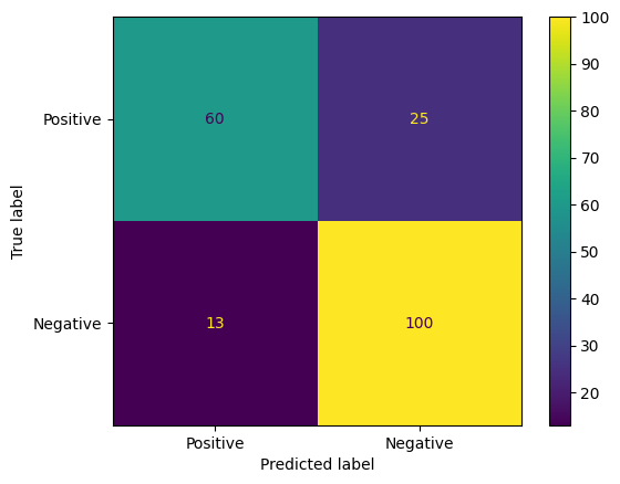
Model tahminlerini değerlendirmenin ilginç bir başka yolu da karışıklık matrisleridir. Karıştırma matrisi, farklı tahmin hatalarını görsel olarak gösterir.
from sklearn.metrics import confusion_matrix, ConfusionMatrixDisplay

cm = confusion_matrix(y_true, y_pred)
ConfusionMatrixDisplay(
    confusion_matrix=cm,
    display_labels=agile_classifier.labels,
).plot()
<sklearn.metrics._plot.confusion_matrix.ConfusionMatrixDisplay at 0x7eb7e2d29ab0>
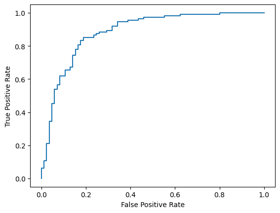
Son olarak, farklı puanlama eşikleri kullanırken olası tahmin hatalarını anlamak için ROC eğrisine de bakabilirsiniz.
from sklearn.metrics import RocCurveDisplay, roc_curve

fpr, tpr, _ = roc_curve(y_true, y_prob, pos_label=1)
RocCurveDisplay(fpr=fpr, tpr=tpr).plot()
<sklearn.metrics._plot.roc_curve.RocCurveDisplay at 0x7eb4d130ef20>
Ek
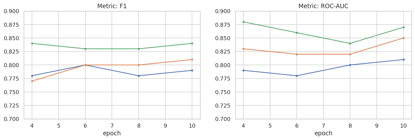
Veri kümesi boyutu ile performans arasındaki ilişkiyi daha iyi anlamak için hiper parametre alanında bazı temel keşifler yaptık. Aşağıdaki grafiğe bakın.
import matplotlib.pyplot as plt
import pandas as pd
import seaborn as sns

sns.set_theme(style="whitegrid")

results_f1 = pd.DataFrame([
    {'training_size': 800, 'epoch': 4, 'metric': 'f1', 'score': 0.84},
    {'training_size': 800, 'epoch': 6, 'metric': 'f1', 'score': 0.83},
    {'training_size': 800, 'epoch': 8, 'metric': 'f1', 'score': 0.83},
    {'training_size': 800, 'epoch': 10, 'metric': 'f1', 'score': 0.84},
    {'training_size': 400, 'epoch': 4, 'metric': 'f1', 'score': 0.77},
    {'training_size': 400, 'epoch': 6, 'metric': 'f1', 'score': 0.80},
    {'training_size': 400, 'epoch': 8, 'metric': 'f1', 'score': 0.80},
    {'training_size': 400, 'epoch': 10,'metric': 'f1', 'score': 0.81},
    {'training_size': 200, 'epoch': 4, 'metric': 'f1', 'score': 0.78},
    {'training_size': 200, 'epoch': 6, 'metric': 'f1', 'score': 0.80},
    {'training_size': 200, 'epoch': 8, 'metric': 'f1', 'score': 0.78},
    {'training_size': 200, 'epoch': 10, 'metric': 'f1', 'score': 0.79},
])

results_roc_auc = pd.DataFrame([
    {'training_size': 800, 'epoch': 4, 'metric': 'roc-auc', 'score': 0.88},
    {'training_size': 800, 'epoch': 6, 'metric': 'roc-auc', 'score': 0.86},
    {'training_size': 800, 'epoch': 8, 'metric': 'roc-auc', 'score': 0.84},
    {'training_size': 800, 'epoch': 10, 'metric': 'roc-auc', 'score': 0.87},
    {'training_size': 400, 'epoch': 4, 'metric': 'roc-auc', 'score': 0.83},
    {'training_size': 400, 'epoch': 6, 'metric': 'roc-auc', 'score': 0.82},
    {'training_size': 400, 'epoch': 8, 'metric': 'roc-auc', 'score': 0.82},
    {'training_size': 400, 'epoch': 10,'metric': 'roc-auc', 'score': 0.85},
    {'training_size': 200, 'epoch': 4, 'metric': 'roc-auc', 'score': 0.79},
    {'training_size': 200, 'epoch': 6, 'metric': 'roc-auc', 'score': 0.78},
    {'training_size': 200, 'epoch': 8, 'metric': 'roc-auc', 'score': 0.80},
    {'training_size': 200, 'epoch': 10, 'metric': 'roc-auc', 'score': 0.81},
])


plot_opts = dict(style='.-', ylim=(0.7, 0.9))
fig, (ax1, ax2) = plt.subplots(1, 2, figsize=(14, 4))
process_results_df = lambda df: df.set_index('epoch').groupby('training_size')['score']
process_results_df(results_f1).plot(title='Metric: F1', ax=ax1, **plot_opts)
process_results_df(results_roc_auc).plot(title='Metric: ROC-AUC', ax=ax2, **plot_opts)
fig.show()