|
|
|
 عرض المصدر على GitHub عرض المصدر على GitHub
|
|
يوضّح هذا الدرس التطبيقي كيفية إنشاء مصنِّف مخصّص للنصوص باستخدام الضبط الفعال للمعلَمات (PET). بدلاً من تحسين النموذج بالكامل، لا تعدّل طُرق PET سوى عدد صغير من المَعلمات، ما يجعل تدريب النموذج سهلًا نسبيًا وسريعًا. ويسهّل ذلك أيضًا على النموذج تعلُّم سلوكيات جديدة باستخدام بيانات تدريب قليلة نسبيًا. تم وصف المنهجية بالتفصيل في مقالة Towards Agile Text Classifiers for Everyone التي توضّح كيفية تطبيق هذه الأساليب على مجموعة متنوعة من مهام السلامة وتحقيق أفضل أداء باستخدام بضع مئات من أمثلة التدريب فقط.
يستخدم هذا الدليل التعليمي لكتابة الرموز البرمجية طريقة الضبط الفعال للمعلَمات (PET) في LoRA
ونموذج Gemma الأصغر حجمًا (gemma_instruct_2b_en) لأنّه يمكن تشغيله بشكل أسرع
وبكفاءة أكبر. يتناول هذا المشروع التعاوني خطوات نقل البيانات وتنسيقها
للنموذج اللغوي الكبير وتدريب أوزان LoRA ثم تقييم النتائج. يتم تدريب
هذا الرمز البرمجي على مجموعة بيانات ETHOS، وهي مجموعة بيانات متوفرة للجميع
لرصد الكلام الذي يحض على الكراهية، وتم إنشاؤها من تعليقات YouTube وReddit.
عند تدريبه على 200 مثال فقط (ربع مجموعة البيانات)، يحقّق هذا النموذج قيمة F1: 0.80 و
ROC-AUC: 0.78، أي أعلى بقليل من أفضل الحلول الحالية المُسجّلة في
قائمة الصدارة (في وقت كتابة هذه المقالة، 15 شباط (فبراير) 2024). عند
تدريبه على العدد الكامل من الأمثلة الـ 800، يحقّق مقياس دقة الاختبار 83.74 وقياس AUC-ROC 88.17. إنّ النماذج الأكبر حجمًا، مثل gemma_instruct_7b_en، ستحقق عمومًا أداءً أفضل، ولكن تكاليف التدريب والتنفيذ ستكون أكبر أيضًا.
تحذير: بما أنّ هذا الدليل التعليمي لإنشاء البرامج يطوّر مصنّف أمان لتحديد الكلام الذي يحض على الكراهية، تحتوي الأمثلة وتقييم النتائج على بعض الكلمات البذيئة.
التثبيت والإعداد
في هذا الدليل التعليمي حول رموز البرامج، ستحتاج إلى إصدار حديث من keras (3) وkeras-nlp
(0.8.0) وحساب على Kaggle لتنزيل نموذج Gemma.
import kagglehub

kagglehub.login()
pip install -q -U keras-nlppip install -q -U keras
import os

os.environ["KERAS_BACKEND"] = "tensorflow"
تحميل مجموعة بيانات ETHOS
في هذا القسم، ستحمِّل مجموعة البيانات التي سيتم تدريب المصنِّف عليها، ثم تتم معالجتها مسبقًا لتصبح مجموعة تدريب ومجموعة اختبار. ستستخدم مجموعة بيانات البحث الرائجة ETHOS التي تم جمعها لرصد الكلام الذي يحض على الكراهية في وسائل التواصل الاجتماعي. يمكنك قراءة المزيد من المعلومات حول كيفية جمع مجموعة البيانات في المقالة ETHOS: an Online Hate Speech Detection Dataset.
import pandas as pd

gh_root = 'https://raw.githubusercontent.com'
gh_repo = 'intelligence-csd-auth-gr/Ethos-Hate-Speech-Dataset'
gh_path = 'master/ethos/ethos_data/Ethos_Dataset_Binary.csv'
data_url = f'{gh_root}/{gh_repo}/{gh_path}'

df = pd.read_csv(data_url, delimiter=';')
df['hateful'] = (df['isHate'] >= df['isHate'].median()).astype(int)

# Shuffle the dataset.
df = df.sample(frac=1, random_state=32)

# Split into train and test.
df_train, df_test = df[:800],  df[800:]

# Display a sample of the data.
df.head(5)[['hateful', 'comment']]
تنزيل النموذج وإنشاء مثيل له
كما هو موضّح في المستندات، يمكنك بسهولة استخدام نموذج Gemma بعدة طرق. في Keras، عليك اتّباع الخطوات التالية:
import keras
import keras_nlp

# For reproducibility purposes.
keras.utils.set_random_seed(1234)

# Download the model from Kaggle using Keras.
model = keras_nlp.models.GemmaCausalLM.from_preset('gemma_instruct_2b_en')

# Set the sequence length to a small enough value to fit in memory in Colab.
model.preprocessor.sequence_length = 128
model.generate('Question: what is the capital of France? ', max_length=32)
معالجة النصوص المُسبَقة ورموز الفواصل
لمساعدة النموذج في فهم القصد بشكل أفضل، يمكنك إجراء معالجة مسبقة للنص و استخدام الرموز المميّزة للفاصل. ويقلّل ذلك من احتمال أن ينشئ النموذج نصًا لا يناسب التنسيق المتوقّع. على سبيل المثال، يمكنك محاولة طلب تصنيف المشاعر من النموذج من خلال كتابة طلب مثل هذا:
Classify the following text into one of the following classes:[Positive,Negative]

Text: you look very nice today
Classification:
في هذه الحالة، قد يعرض النموذج ما تبحث عنه أو لا يعرضه. على سبيل المثال، إذا كان النص يحتوي على أحرف سطر جديد، من المرجّح أن يؤثر ذلك سلبًا في أداء النموذج. هناك طريقة أكثر فعالية وهي استخدام فاصل العلامات. تصبح المطالبة بعد ذلك:
Classify the following text into one of the following classes:[Positive,Negative]
<separator>
Text: you look very nice today
<separator>
Prediction:
ويمكن تبسيط ذلك باستخدام دالة تعالج النص مسبقًا:
def preprocess_text(
    text: str,
    labels: list[str],
    instructions: str,
    separator: str,
) -> str:
  prompt = f'{instructions}:[{",".join(labels)}]'
  return separator.join([prompt, f'Text:{text}', 'Prediction:'])
الآن، إذا نفّذت الدالة باستخدام الطلب والنص نفسهما كما في السابق، من المفترض أن تحصل على الإخراج نفسه:
text = 'you look very nice today'

prompt = preprocess_text(
    text=text,
    labels=['Positive', 'Negative'],
    instructions='Classify the following text into one of the following classes',
    separator='\n<separator>\n',
)

print(prompt)
Classify the following text into one of the following classes:[Positive,Negative]
<separator>
Text:you look very nice today
<separator>
Prediction:
المعالجة اللاحقة للإخراج
مخرجات النموذج هي الرموز التي تتضمّن احتمالات مختلفة. عادةً، لمحاولة
إنشاء نص، عليك الاختيار من بين أهم الرموز القليلة الأكثر احتمالًا
ومحاولة إنشاء جمل أو فقرات أو حتى مستندات كاملة. ومع ذلك، لأغراض
التصنيف، ما يهمّ فعلاً هو ما إذا كان النموذج يعتقد أنّ احتمال وقوع
Positive أكبر من احتمال وقوع Negative أو العكس.
استنادًا إلى النموذج الذي أنشأته سابقًا، في ما يلي كيفية معالجة ناتجه
إلى الاحتمالات المستقلة لحدوث الرمز المميّز التالي Positive أو
Negative، على التوالي:
import numpy as np


def compute_output_probability(
    model: keras_nlp.models.GemmaCausalLM,
    prompt: str,
    target_classes: list[str],
) -> dict[str, float]:
  # Shorthands.
  preprocessor = model.preprocessor
  tokenizer = preprocessor.tokenizer

  # NOTE: If a token is not found, it will be considered same as "<unk>".
  token_unk = tokenizer.token_to_id('<unk>')

  # Identify the token indices, which is the same as the ID for this tokenizer.
  token_ids = [tokenizer.token_to_id(word) for word in target_classes]

  # Throw an error if one of the classes maps to a token outside the vocabulary.
  if any(token_id == token_unk for token_id in token_ids):
    raise ValueError('One of the target classes is not in the vocabulary.')

  # Preprocess the prompt in a single batch. This is done one sample at a time
  # for illustration purposes, but it would be more efficient to batch prompts.
  preprocessed = model.preprocessor.generate_preprocess([prompt])

  # Identify output token offset.
  padding_mask = preprocessed["padding_mask"]
  token_offset = keras.ops.sum(padding_mask) - 1

  # Score outputs, extract only the next token's logits.
  vocab_logits = model.score(
      token_ids=preprocessed["token_ids"],
      padding_mask=padding_mask,
  )[0][token_offset]

  # Compute the relative probability of each of the requested tokens.
  token_logits = [vocab_logits[ix] for ix in token_ids]
  logits_tensor = keras.ops.convert_to_tensor(token_logits)
  probabilities = keras.activations.softmax(logits_tensor)

  return dict(zip(target_classes, probabilities.numpy()))
يمكنك اختبار هذه الدالة من خلال تشغيلها مع الطلب الذي أنشأته سابقًا:
compute_output_probability(
    model=model,
    prompt=prompt,
    target_classes=['Positive', 'Negative'],
)
{'Positive': 0.99994016, 'Negative': 5.984089e-05}
تلخيص كلّ ذلك على أنّه مصنّف
لتسهيل الاستخدام، يمكنك تجميع جميع الدوال التي أنشأتها للتو في
تصنيف واحد مثل sklearn باستخدام دوال سهلة الاستخدام ومألوفة مثل
predict() وpredict_score().
import dataclasses


@dataclasses.dataclass(frozen=True)
class AgileClassifier:
  """Agile classifier to be wrapped around a LLM."""

  # The classes whose probability will be predicted.
  labels: tuple[str, ...]

  # Provide default instructions and control tokens, can be overridden by user.
  instructions: str = 'Classify the following text into one of the following classes'
  separator_token: str = '<separator>'
  end_of_text_token: str = '<eos>'

  def encode_for_prediction(self, x_text: str) -> str:
    return preprocess_text(
        text=x_text,
        labels=self.labels,
        instructions=self.instructions,
        separator=self.separator_token,
    )

  def encode_for_training(self, x_text: str, y: int) -> str:
    return ''.join([
        self.encode_for_prediction(x_text),
        self.labels[y],
        self.end_of_text_token,
    ])

  def predict_score(
      self,
      model: keras_nlp.models.GemmaCausalLM,
      x_text: str,
  ) -> list[float]:
    prompt = self.encode_for_prediction(x_text)
    token_probabilities = compute_output_probability(
        model=model,
        prompt=prompt,
        target_classes=self.labels,
    )
    return [token_probabilities[token] for token in self.labels]

  def predict(
      self,
      model: keras_nlp.models.GemmaCausalLM,
      x_eval: str,
  ) -> int:
    return np.argmax(self.predict_score(model, x_eval))

agile_classifier = AgileClassifier(labels=('Positive', 'Negative'))
تحسين النموذج
يشير اختصار LoRA إلى Low-Rank Adaptation (التأقلم منخفضة الترتيب). وهي تقنية تحسين يمكن استخدامها لتحسين النماذج اللغوية الكبيرة بكفاءة. يمكنك الاطّلاع على مزيد من المعلومات عنه في مقالة LoRA: Low-Rank Adaptation of Large Language Models.
يقدّم تطبيق Keras لنموذج Gemma طريقة enable_lora() يمكنك
استخدامها للتحسين:
# Enable LoRA for the model and set the LoRA rank to 4.
model.backbone.enable_lora(rank=4)
بعد تفعيل LoRA، يمكنك بدء عملية التحسين. يستغرق ذلك 5 دقائق تقريبًا لكل دورة تدريب على Colab:
import tensorflow as tf

# Create dataset with preprocessed text + labels.
map_fn = lambda x: agile_classifier.encode_for_training(*x)
x_train = list(map(map_fn, df_train[['comment', 'hateful']].values))
ds_train = tf.data.Dataset.from_tensor_slices(x_train).batch(2)

# Compile the model using the Adam optimizer and appropriate loss function.
model.compile(
    loss=keras.losses.SparseCategoricalCrossentropy(from_logits=True),
    optimizer=keras.optimizers.Adam(learning_rate=0.0005),
    weighted_metrics=[keras.metrics.SparseCategoricalAccuracy()],
)

# Begin training.
model.fit(ds_train, epochs=4)
Epoch 1/4
400/400 ━━━━━━━━━━━━━━━━━━━━ 354s 703ms/step - loss: 1.1365 - sparse_categorical_accuracy: 0.5874
Epoch 2/4
400/400 ━━━━━━━━━━━━━━━━━━━━ 338s 716ms/step - loss: 0.7579 - sparse_categorical_accuracy: 0.6662
Epoch 3/4
400/400 ━━━━━━━━━━━━━━━━━━━━ 324s 721ms/step - loss: 0.6818 - sparse_categorical_accuracy: 0.6894
Epoch 4/4
400/400 ━━━━━━━━━━━━━━━━━━━━ 323s 725ms/step - loss: 0.5922 - sparse_categorical_accuracy: 0.7220
<keras.src.callbacks.history.History at 0x7eb7e369c490>
سيؤدي التدريب لعدد أكبر من الفترات إلى تحقيق دقة أعلى، إلى أن يحدث التطابق المفرط.
فحص النتائج
يمكنك الآن فحص ناتج المصنّف السريع الذي تدرّبت عليه للتو. سيعرض هذا الرمز نتيجة الصف المتوقّعة استنادًا إلى جزء من النص:
text = 'you look really nice today'
scores = agile_classifier.predict_score(model, text)
dict(zip(agile_classifier.labels, scores))
{'Positive': 0.99899644, 'Negative': 0.0010035498}
تقييم النموذج
أخيرًا، ستقيّم أداء النموذج باستخدام مقياسَين شائعَين، وهوَين مقياس F1 وAUC-ROC. يرصد مقياس دقة الاختبار أخطاء التقييمات العميقةالسلبية والموجبة الخاطئة من خلال تقييم المتوسط التوافقي لدقةالتقييم واكتمال التوقعات الإيجابية عند حدّ معيّن للتصنيف. من ناحية أخرى، يرصد مقياس AUC-ROC التوازن بين معدّل الموجب الصحيح ومعدّل الموجب الخاطئ على مستوى مجموعة متنوّعة من الحدود الدنيا ويحسب المساحة تحت هذا المنحنى.
y_true = df_test['hateful'].values
# Compute the scores (aka probabilities) for each of the labels.
y_score = [agile_classifier.predict_score(model, x) for x in df_test['comment']]
# The label with highest score is considered the predicted class.
y_pred = np.argmax(y_score, axis=1)
# Extract the probability of a comment being considered hateful.
y_prob = [x[agile_classifier.labels.index('Negative')] for x in y_score]
from sklearn.metrics import f1_score, roc_auc_score

print(f'F1: {f1_score(y_true, y_pred):.2f}')
print(f'AUC-ROC: {roc_auc_score(y_true, y_prob):.2f}')
F1: 0.84
AUC-ROC: 0.88
هناك طريقة أخرى مثيرة للاهتمام لتقييم توقّعات النماذج وهي مصفوفات الالتباس. ستعرض مصفوفة الالتباس أنواع الأخطاء المختلفة في التوقّعات بشكل مرئي.
from sklearn.metrics import confusion_matrix, ConfusionMatrixDisplay

cm = confusion_matrix(y_true, y_pred)
ConfusionMatrixDisplay(
    confusion_matrix=cm,
    display_labels=agile_classifier.labels,
).plot()
<sklearn.metrics._plot.confusion_matrix.ConfusionMatrixDisplay at 0x7eb7e2d29ab0>

أخيرًا، يمكنك أيضًا الاطّلاع على منحنى ROC لمعرفة أخطاء التنبؤ المحتملة عند استخدام عتبات تقييم مختلفة.
from sklearn.metrics import RocCurveDisplay, roc_curve

fpr, tpr, _ = roc_curve(y_true, y_prob, pos_label=1)
RocCurveDisplay(fpr=fpr, tpr=tpr).plot()
<sklearn.metrics._plot.roc_curve.RocCurveDisplay at 0x7eb4d130ef20>

الملحق
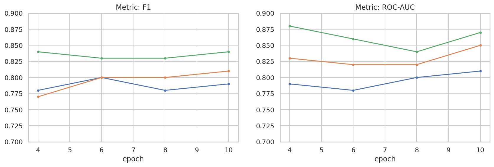
لقد أجرينا بعض الاستكشافات الأساسية لمساحة المَعلمات الفائقة للمساعدة في فهم العلاقة بين حجم مجموعة البيانات والأداء بشكل أفضل. اطّلِع على الرسم البياني التالي.
import matplotlib.pyplot as plt
import pandas as pd
import seaborn as sns

sns.set_theme(style="whitegrid")

results_f1 = pd.DataFrame([
    {'training_size': 800, 'epoch': 4, 'metric': 'f1', 'score': 0.84},
    {'training_size': 800, 'epoch': 6, 'metric': 'f1', 'score': 0.83},
    {'training_size': 800, 'epoch': 8, 'metric': 'f1', 'score': 0.83},
    {'training_size': 800, 'epoch': 10, 'metric': 'f1', 'score': 0.84},
    {'training_size': 400, 'epoch': 4, 'metric': 'f1', 'score': 0.77},
    {'training_size': 400, 'epoch': 6, 'metric': 'f1', 'score': 0.80},
    {'training_size': 400, 'epoch': 8, 'metric': 'f1', 'score': 0.80},
    {'training_size': 400, 'epoch': 10,'metric': 'f1', 'score': 0.81},
    {'training_size': 200, 'epoch': 4, 'metric': 'f1', 'score': 0.78},
    {'training_size': 200, 'epoch': 6, 'metric': 'f1', 'score': 0.80},
    {'training_size': 200, 'epoch': 8, 'metric': 'f1', 'score': 0.78},
    {'training_size': 200, 'epoch': 10, 'metric': 'f1', 'score': 0.79},
])

results_roc_auc = pd.DataFrame([
    {'training_size': 800, 'epoch': 4, 'metric': 'roc-auc', 'score': 0.88},
    {'training_size': 800, 'epoch': 6, 'metric': 'roc-auc', 'score': 0.86},
    {'training_size': 800, 'epoch': 8, 'metric': 'roc-auc', 'score': 0.84},
    {'training_size': 800, 'epoch': 10, 'metric': 'roc-auc', 'score': 0.87},
    {'training_size': 400, 'epoch': 4, 'metric': 'roc-auc', 'score': 0.83},
    {'training_size': 400, 'epoch': 6, 'metric': 'roc-auc', 'score': 0.82},
    {'training_size': 400, 'epoch': 8, 'metric': 'roc-auc', 'score': 0.82},
    {'training_size': 400, 'epoch': 10,'metric': 'roc-auc', 'score': 0.85},
    {'training_size': 200, 'epoch': 4, 'metric': 'roc-auc', 'score': 0.79},
    {'training_size': 200, 'epoch': 6, 'metric': 'roc-auc', 'score': 0.78},
    {'training_size': 200, 'epoch': 8, 'metric': 'roc-auc', 'score': 0.80},
    {'training_size': 200, 'epoch': 10, 'metric': 'roc-auc', 'score': 0.81},
])


plot_opts = dict(style='.-', ylim=(0.7, 0.9))
fig, (ax1, ax2) = plt.subplots(1, 2, figsize=(14, 4))
process_results_df = lambda df: df.set_index('epoch').groupby('training_size')['score']
process_results_df(results_f1).plot(title='Metric: F1', ax=ax1, **plot_opts)
process_results_df(results_roc_auc).plot(title='Metric: ROC-AUC', ax=ax2, **plot_opts)
fig.show()