|
|
|
 GitHub에서 소스 보기 GitHub에서 소스 보기
|
|
이 Codelab에서는 파라미터 효율적인 튜닝 (PET)을 사용하여 맞춤설정된 텍스트 분류기를 만드는 방법을 보여줍니다. PET 메서드는 전체 모델을 미세 조정하는 대신 소량의 매개변수만 업데이트하므로 비교적 쉽고 빠르게 학습할 수 있습니다. 또한 모델이 비교적 적은 양의 학습 데이터로 새로운 동작을 더 쉽게 학습할 수 있습니다. 이 방법론은 모든 사용자를 위한 민첩한 텍스트 분류기에서 자세히 설명합니다. 이 방법론에서는 이러한 기법을 다양한 안전 작업에 적용하고 수백 개의 학습 예시만으로 최신 성능을 달성하는 방법을 보여줍니다.
이 Codelab에서는 더 빠르고 효율적으로 실행할 수 있는 LoRA PET 메서드와 더 작은 Gemma 모델 (gemma_instruct_2b_en)을 사용합니다. 이 colab에서는 데이터를 처리하고, LLM에 맞게 형식을 지정하고, LoRA 가중치를 학습한 후 결과를 평가하는 단계를 다룹니다. 이 Codelab에서는 YouTube 및 Reddit 댓글에서 구축된 증오심 표현 감지를 위한 공개 데이터 세트인 ETHOS 데이터 세트를 학습합니다.
200개 예시 (데이터 세트의 1/4)로만 학습하면 F1: 0.80, ROC-AUC: 0.78을 달성하여 현재 리더보드에 보고된 SOTA (작성 당시: 2024년 2월 15일)보다 약간 높습니다. 전체 800개 예시로 학습하면 F1 점수 83.74, ROC-AUC 점수 88.17을 달성합니다. gemma_instruct_7b_en와 같이 더 큰 모델은 일반적으로 성능이 더 우수하지만 학습 및 실행 비용도 더 큽니다.
트리거 경고: 이 Codelab에서는 증오심 표현을 감지하기 위한 안전 분류기를 개발하므로 결과의 예시와 평가에 끔찍한 표현이 포함되어 있습니다.
설치 및 설정
이 Codelab에서는 최신 버전 keras (3), keras-nlp(0.8.0)과 Kaggle 계정이 필요하며, 이를 사용하여 Gemma 모델을 다운로드합니다.
import kagglehub

kagglehub.login()
pip install -q -U keras-nlppip install -q -U keras
import os

os.environ["KERAS_BACKEND"] = "tensorflow"
ETHOS 데이터 세트 로드
이 섹션에서는 분류기를 학습할 데이터 세트를 로드하고 학습 및 테스트 세트로 사전 처리합니다. 소셜 미디어에서 증오심 표현을 감지하기 위해 수집된 인기 있는 연구 데이터 세트인 ETHOS를 사용합니다. 데이터 세트 수집 방법에 관한 자세한 내용은 ETHOS: 온라인 증오심 표현 감지 데이터 세트 논문을 참고하세요.
import pandas as pd

gh_root = 'https://raw.githubusercontent.com'
gh_repo = 'intelligence-csd-auth-gr/Ethos-Hate-Speech-Dataset'
gh_path = 'master/ethos/ethos_data/Ethos_Dataset_Binary.csv'
data_url = f'{gh_root}/{gh_repo}/{gh_path}'

df = pd.read_csv(data_url, delimiter=';')
df['hateful'] = (df['isHate'] >= df['isHate'].median()).astype(int)

# Shuffle the dataset.
df = df.sample(frac=1, random_state=32)

# Split into train and test.
df_train, df_test = df[:800],  df[800:]

# Display a sample of the data.
df.head(5)[['hateful', 'comment']]
모델 다운로드 및 인스턴스화
문서에 설명된 대로 다양한 방법으로 Gemma 모델을 쉽게 사용할 수 있습니다. Keras를 사용하려면 다음 단계를 따르세요.
import keras
import keras_nlp

# For reproducibility purposes.
keras.utils.set_random_seed(1234)

# Download the model from Kaggle using Keras.
model = keras_nlp.models.GemmaCausalLM.from_preset('gemma_instruct_2b_en')

# Set the sequence length to a small enough value to fit in memory in Colab.
model.preprocessor.sequence_length = 128
model.generate('Question: what is the capital of France? ', max_length=32)
텍스트 전처리 및 구분자 토큰
모델이 의도를 더 잘 이해할 수 있도록 텍스트를 사전 처리하고 구분자 토큰을 사용할 수 있습니다. 이렇게 하면 모델이 예상 형식에 맞지 않는 텍스트를 생성할 가능성이 줄어듭니다. 예를 들어 다음과 같은 프롬프트를 작성하여 모델에 감정 분류를 요청할 수 있습니다.
Classify the following text into one of the following classes:[Positive,Negative]

Text: you look very nice today
Classification:
이 경우 모델이 원하는 결과를 출력할 수도 있고 그렇지 않을 수도 있습니다. 예를 들어 텍스트에 줄바꿈 문자가 포함되어 있으면 모델 성능에 부정적인 영향을 미칠 수 있습니다. 더 강력한 접근 방식은 구분자 토큰을 사용하는 것입니다. 그러면 프롬프트가 다음과 같이 변경됩니다.
Classify the following text into one of the following classes:[Positive,Negative]
<separator>
Text: you look very nice today
<separator>
Prediction:
텍스트를 전처리하는 함수를 사용하여 추상화할 수 있습니다.
def preprocess_text(
    text: str,
    labels: list[str],
    instructions: str,
    separator: str,
) -> str:
  prompt = f'{instructions}:[{",".join(labels)}]'
  return separator.join([prompt, f'Text:{text}', 'Prediction:'])
이제 이전과 동일한 프롬프트와 텍스트를 사용하여 함수를 실행하면 동일한 출력이 표시됩니다.
text = 'you look very nice today'

prompt = preprocess_text(
    text=text,
    labels=['Positive', 'Negative'],
    instructions='Classify the following text into one of the following classes',
    separator='\n<separator>\n',
)

print(prompt)
Classify the following text into one of the following classes:[Positive,Negative]
<separator>
Text:you look very nice today
<separator>
Prediction:
출력 후처리
모델의 출력은 다양한 확률을 가진 토큰입니다. 일반적으로 텍스트를 생성하려면 가장 확률이 높은 몇 개의 토큰 중에서 선택하고 문장, 단락 또는 전체 문서를 구성합니다. 그러나 분류의 목적으로는 모델이 Positive가 Negative보다 가능성이 더 높다고 생각하는지가 실제로 중요합니다.
앞서 인스턴스화한 모델을 고려할 때 다음 토큰이 각각 Positive인지 Negative인지에 대한 독립적인 확률로 출력을 처리하는 방법은 다음과 같습니다.
import numpy as np


def compute_output_probability(
    model: keras_nlp.models.GemmaCausalLM,
    prompt: str,
    target_classes: list[str],
) -> dict[str, float]:
  # Shorthands.
  preprocessor = model.preprocessor
  tokenizer = preprocessor.tokenizer

  # NOTE: If a token is not found, it will be considered same as "<unk>".
  token_unk = tokenizer.token_to_id('<unk>')

  # Identify the token indices, which is the same as the ID for this tokenizer.
  token_ids = [tokenizer.token_to_id(word) for word in target_classes]

  # Throw an error if one of the classes maps to a token outside the vocabulary.
  if any(token_id == token_unk for token_id in token_ids):
    raise ValueError('One of the target classes is not in the vocabulary.')

  # Preprocess the prompt in a single batch. This is done one sample at a time
  # for illustration purposes, but it would be more efficient to batch prompts.
  preprocessed = model.preprocessor.generate_preprocess([prompt])

  # Identify output token offset.
  padding_mask = preprocessed["padding_mask"]
  token_offset = keras.ops.sum(padding_mask) - 1

  # Score outputs, extract only the next token's logits.
  vocab_logits = model.score(
      token_ids=preprocessed["token_ids"],
      padding_mask=padding_mask,
  )[0][token_offset]

  # Compute the relative probability of each of the requested tokens.
  token_logits = [vocab_logits[ix] for ix in token_ids]
  logits_tensor = keras.ops.convert_to_tensor(token_logits)
  probabilities = keras.activations.softmax(logits_tensor)

  return dict(zip(target_classes, probabilities.numpy()))
이전에 만든 프롬프트로 함수를 실행하여 테스트할 수 있습니다.
compute_output_probability(
    model=model,
    prompt=prompt,
    target_classes=['Positive', 'Negative'],
)
{'Positive': 0.99994016, 'Negative': 5.984089e-05}
분류자로 모든 것을 래핑
사용 편의를 위해 방금 만든 모든 함수를 predict() 및 predict_score()와 같이 사용하기 쉽고 익숙한 함수를 사용하여 단일 sklearn과 유사한 분류기로 래핑할 수 있습니다.
import dataclasses


@dataclasses.dataclass(frozen=True)
class AgileClassifier:
  """Agile classifier to be wrapped around a LLM."""

  # The classes whose probability will be predicted.
  labels: tuple[str, ...]

  # Provide default instructions and control tokens, can be overridden by user.
  instructions: str = 'Classify the following text into one of the following classes'
  separator_token: str = '<separator>'
  end_of_text_token: str = '<eos>'

  def encode_for_prediction(self, x_text: str) -> str:
    return preprocess_text(
        text=x_text,
        labels=self.labels,
        instructions=self.instructions,
        separator=self.separator_token,
    )

  def encode_for_training(self, x_text: str, y: int) -> str:
    return ''.join([
        self.encode_for_prediction(x_text),
        self.labels[y],
        self.end_of_text_token,
    ])

  def predict_score(
      self,
      model: keras_nlp.models.GemmaCausalLM,
      x_text: str,
  ) -> list[float]:
    prompt = self.encode_for_prediction(x_text)
    token_probabilities = compute_output_probability(
        model=model,
        prompt=prompt,
        target_classes=self.labels,
    )
    return [token_probabilities[token] for token in self.labels]

  def predict(
      self,
      model: keras_nlp.models.GemmaCausalLM,
      x_eval: str,
  ) -> int:
    return np.argmax(self.predict_score(model, x_eval))

agile_classifier = AgileClassifier(labels=('Positive', 'Negative'))
모델 미세 조정
LoRA는 Low-Rank Adaptation의 약자입니다. 대규모 언어 모델을 효율적으로 미세 조정하는 데 사용할 수 있는 미세 조정 기법입니다. LoRA: 대규모 언어 모델의 하위 순위 조정 논문에서 자세히 알아보세요.
Gemma의 Keras 구현은 미세 조정에 사용할 수 있는 enable_lora() 메서드를 제공합니다.
# Enable LoRA for the model and set the LoRA rank to 4.
model.backbone.enable_lora(rank=4)
LoRA를 사용 설정한 후에는 미세 조정 프로세스를 시작할 수 있습니다. Colab에서는 에포크당 약 5분이 소요됩니다.
import tensorflow as tf

# Create dataset with preprocessed text + labels.
map_fn = lambda x: agile_classifier.encode_for_training(*x)
x_train = list(map(map_fn, df_train[['comment', 'hateful']].values))
ds_train = tf.data.Dataset.from_tensor_slices(x_train).batch(2)

# Compile the model using the Adam optimizer and appropriate loss function.
model.compile(
    loss=keras.losses.SparseCategoricalCrossentropy(from_logits=True),
    optimizer=keras.optimizers.Adam(learning_rate=0.0005),
    weighted_metrics=[keras.metrics.SparseCategoricalAccuracy()],
)

# Begin training.
model.fit(ds_train, epochs=4)
Epoch 1/4
400/400 ━━━━━━━━━━━━━━━━━━━━ 354s 703ms/step - loss: 1.1365 - sparse_categorical_accuracy: 0.5874
Epoch 2/4
400/400 ━━━━━━━━━━━━━━━━━━━━ 338s 716ms/step - loss: 0.7579 - sparse_categorical_accuracy: 0.6662
Epoch 3/4
400/400 ━━━━━━━━━━━━━━━━━━━━ 324s 721ms/step - loss: 0.6818 - sparse_categorical_accuracy: 0.6894
Epoch 4/4
400/400 ━━━━━━━━━━━━━━━━━━━━ 323s 725ms/step - loss: 0.5922 - sparse_categorical_accuracy: 0.7220
<keras.src.callbacks.history.History at 0x7eb7e369c490>
과적합이 발생할 때까지 더 많은 에포크를 학습하면 정확성이 높아집니다.
결과 검사
이제 방금 학습한 민첩한 분류기의 출력을 검사할 수 있습니다. 이 코드는 텍스트가 주어지면 예측된 클래스 점수를 출력합니다.
text = 'you look really nice today'
scores = agile_classifier.predict_score(model, text)
dict(zip(agile_classifier.labels, scores))
{'Positive': 0.99899644, 'Negative': 0.0010035498}
모델 평가
마지막으로 두 가지 일반적인 측정항목인 F1 점수와 AUC-ROC를 사용하여 모델의 성능을 평가합니다. F1 점수는 특정 분류 기준점에서 정밀도와 재현율의 조화 평균을 평가하여 거짓음성 및 거짓양성 오류를 포착합니다. 반면 AUC-ROC는 다양한 기준에서 참양성률과 거짓양성률 간의 균형을 포착하고 이 곡선 아래의 면적을 계산합니다.
y_true = df_test['hateful'].values
# Compute the scores (aka probabilities) for each of the labels.
y_score = [agile_classifier.predict_score(model, x) for x in df_test['comment']]
# The label with highest score is considered the predicted class.
y_pred = np.argmax(y_score, axis=1)
# Extract the probability of a comment being considered hateful.
y_prob = [x[agile_classifier.labels.index('Negative')] for x in y_score]
from sklearn.metrics import f1_score, roc_auc_score

print(f'F1: {f1_score(y_true, y_pred):.2f}')
print(f'AUC-ROC: {roc_auc_score(y_true, y_prob):.2f}')
F1: 0.84
AUC-ROC: 0.88
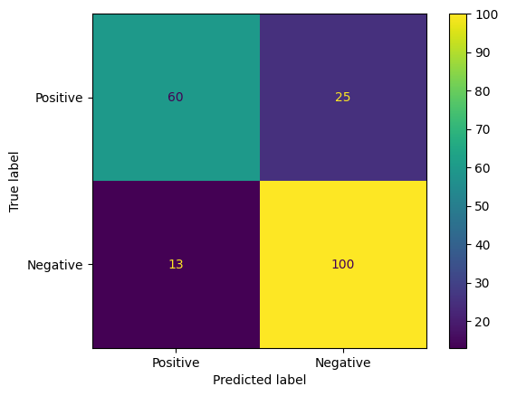
모델 예측을 평가하는 또 다른 흥미로운 방법은 혼동 행렬입니다. 혼동 행렬은 다양한 종류의 예측 오류를 시각적으로 보여줍니다.
from sklearn.metrics import confusion_matrix, ConfusionMatrixDisplay

cm = confusion_matrix(y_true, y_pred)
ConfusionMatrixDisplay(
    confusion_matrix=cm,
    display_labels=agile_classifier.labels,
).plot()
<sklearn.metrics._plot.confusion_matrix.ConfusionMatrixDisplay at 0x7eb7e2d29ab0>
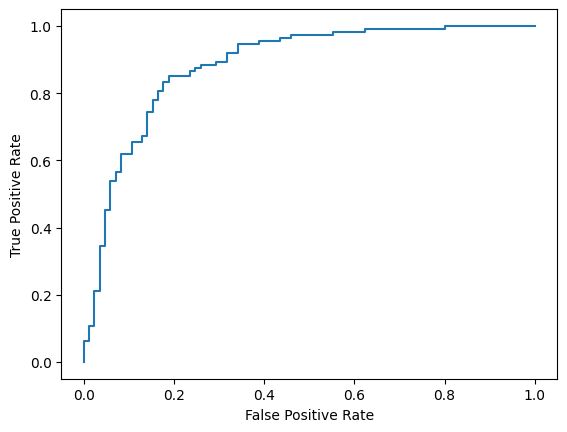
마지막으로 ROC 곡선을 확인하여 다양한 점수 임곗값을 사용할 때의 잠재적 예측 오류를 파악할 수도 있습니다.
from sklearn.metrics import RocCurveDisplay, roc_curve

fpr, tpr, _ = roc_curve(y_true, y_prob, pos_label=1)
RocCurveDisplay(fpr=fpr, tpr=tpr).plot()
<sklearn.metrics._plot.roc_curve.RocCurveDisplay at 0x7eb4d130ef20>
부록
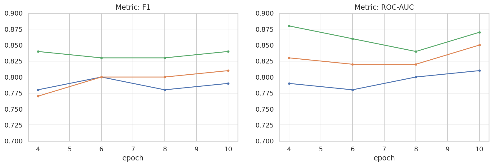
데이터 세트 크기와 실적 간의 관계를 더 잘 이해할 수 있도록 하이퍼파라미터 공간을 기본적으로 살펴봤습니다. 다음 그래프를 참고하세요.
import matplotlib.pyplot as plt
import pandas as pd
import seaborn as sns

sns.set_theme(style="whitegrid")

results_f1 = pd.DataFrame([
    {'training_size': 800, 'epoch': 4, 'metric': 'f1', 'score': 0.84},
    {'training_size': 800, 'epoch': 6, 'metric': 'f1', 'score': 0.83},
    {'training_size': 800, 'epoch': 8, 'metric': 'f1', 'score': 0.83},
    {'training_size': 800, 'epoch': 10, 'metric': 'f1', 'score': 0.84},
    {'training_size': 400, 'epoch': 4, 'metric': 'f1', 'score': 0.77},
    {'training_size': 400, 'epoch': 6, 'metric': 'f1', 'score': 0.80},
    {'training_size': 400, 'epoch': 8, 'metric': 'f1', 'score': 0.80},
    {'training_size': 400, 'epoch': 10,'metric': 'f1', 'score': 0.81},
    {'training_size': 200, 'epoch': 4, 'metric': 'f1', 'score': 0.78},
    {'training_size': 200, 'epoch': 6, 'metric': 'f1', 'score': 0.80},
    {'training_size': 200, 'epoch': 8, 'metric': 'f1', 'score': 0.78},
    {'training_size': 200, 'epoch': 10, 'metric': 'f1', 'score': 0.79},
])

results_roc_auc = pd.DataFrame([
    {'training_size': 800, 'epoch': 4, 'metric': 'roc-auc', 'score': 0.88},
    {'training_size': 800, 'epoch': 6, 'metric': 'roc-auc', 'score': 0.86},
    {'training_size': 800, 'epoch': 8, 'metric': 'roc-auc', 'score': 0.84},
    {'training_size': 800, 'epoch': 10, 'metric': 'roc-auc', 'score': 0.87},
    {'training_size': 400, 'epoch': 4, 'metric': 'roc-auc', 'score': 0.83},
    {'training_size': 400, 'epoch': 6, 'metric': 'roc-auc', 'score': 0.82},
    {'training_size': 400, 'epoch': 8, 'metric': 'roc-auc', 'score': 0.82},
    {'training_size': 400, 'epoch': 10,'metric': 'roc-auc', 'score': 0.85},
    {'training_size': 200, 'epoch': 4, 'metric': 'roc-auc', 'score': 0.79},
    {'training_size': 200, 'epoch': 6, 'metric': 'roc-auc', 'score': 0.78},
    {'training_size': 200, 'epoch': 8, 'metric': 'roc-auc', 'score': 0.80},
    {'training_size': 200, 'epoch': 10, 'metric': 'roc-auc', 'score': 0.81},
])


plot_opts = dict(style='.-', ylim=(0.7, 0.9))
fig, (ax1, ax2) = plt.subplots(1, 2, figsize=(14, 4))
process_results_df = lambda df: df.set_index('epoch').groupby('training_size')['score']
process_results_df(results_f1).plot(title='Metric: F1', ax=ax1, **plot_opts)
process_results_df(results_roc_auc).plot(title='Metric: ROC-AUC', ax=ax2, **plot_opts)
fig.show()