| | |  GitHub-এ উৎস দেখুন GitHub-এ উৎস দেখুন | |
এই কোডল্যাবটি ব্যাখ্যা করে কিভাবে প্যারামিটার দক্ষ টিউনিং (PET) ব্যবহার করে একটি কাস্টমাইজড টেক্সট ক্লাসিফায়ার তৈরি করা যায়। পুরো মডেলকে ফাইন-টিউন করার পরিবর্তে, PET পদ্ধতিগুলি শুধুমাত্র অল্প পরিমাণ প্যারামিটার আপডেট করে, যা এটিকে তুলনামূলকভাবে সহজ এবং দ্রুত প্রশিক্ষণ দেয়। এটি একটি মডেলের জন্য তুলনামূলকভাবে অল্প প্রশিক্ষণ ডেটা সহ নতুন আচরণ শেখা সহজ করে তোলে। পদ্ধতিটি বিশদভাবে বর্ণনা করা হয়েছে Towards Agile Text Classifiers for everyone যা দেখায় কিভাবে এই কৌশলগুলি বিভিন্ন নিরাপত্তা কাজে প্রয়োগ করা যেতে পারে এবং মাত্র কয়েকশ প্রশিক্ষণের উদাহরণ দিয়ে শিল্প কর্মক্ষমতা অর্জন করতে পারে।
এই কোডল্যাবটি LoRA PET পদ্ধতি এবং ছোট জেমা মডেল ( gemma_instruct_2b_en ) ব্যবহার করে কারণ এটি দ্রুত এবং আরও দক্ষতার সাথে চালানো যেতে পারে। কোল্যাব ডেটা ইনজেস্ট করার ধাপগুলি কভার করে, এটি এলএলএম-এর জন্য ফর্ম্যাট করে, LoRA ওজনের প্রশিক্ষণ দেয় এবং তারপর ফলাফলগুলি মূল্যায়ন করে৷ এই কোডল্যাবটি ইউটিউব এবং রেডডিট মন্তব্য থেকে তৈরি ঘৃণাপূর্ণ বক্তৃতা শনাক্ত করার জন্য সর্বজনীনভাবে উপলব্ধ একটি ডেটাসেট, ETHOS ডেটাসেটে প্রশিক্ষণ দেয়৷ শুধুমাত্র 200টি উদাহরণের (ডেটাসেটের 1/4) উপর প্রশিক্ষিত হলে এটি F1: 0.80 এবং ROC-AUC: 0.78 অর্জন করে, বর্তমানে লিডারবোর্ডে রিপোর্ট করা SOTA থেকে সামান্য উপরে (লেখার সময়, 15 ফেব্রুয়ারী 2024)। সম্পূর্ণ 800টি উদাহরণের উপর প্রশিক্ষিত হলে, যেমন এটি একটি F1 স্কোর 83.74 এবং একটি ROC-AUC স্কোর 88.17 অর্জন করে। বড় মডেল, যেমন gemma_instruct_7b_en সাধারণত ভাল পারফর্ম করবে, তবে প্রশিক্ষণ এবং সম্পাদনের খরচও বেশি।
ট্রিগার সতর্কীকরণ : কারণ এই কোডল্যাব ঘৃণ্য বক্তৃতা শনাক্ত করার জন্য একটি নিরাপত্তা শ্রেণীবিভাগ তৈরি করে, উদাহরণ এবং ফলাফলের মূল্যায়নে কিছু ভয়ঙ্কর ভাষা রয়েছে।
ইনস্টলেশন এবং সেটআপ
এই কোডল্যাবের জন্য, আপনার একটি সাম্প্রতিক সংস্করণ keras (3), keras-nlp (0.8.0) এবং একটি জেমা মডেল ডাউনলোড করার জন্য একটি কাগল অ্যাকাউন্টের প্রয়োজন হবে।
import kagglehub

kagglehub.login()
pip install -q -U keras-nlppip install -q -U keras
import os

os.environ["KERAS_BACKEND"] = "tensorflow"
ETHOS ডেটাসেট লোড করুন
এই বিভাগে আপনি ডেটাসেট লোড করবেন যার উপর আমাদের ক্লাসিফায়ারকে প্রশিক্ষণ দিতে হবে এবং এটিকে একটি ট্রেন এবং পরীক্ষা সেটে প্রিপ্রসেস করতে হবে। আপনি জনপ্রিয় গবেষণা ডেটাসেট ETHOS ব্যবহার করবেন যা সামাজিক মিডিয়াতে ঘৃণাত্মক বক্তব্য সনাক্ত করতে সংগ্রহ করা হয়েছিল। কিভাবে ডেটাসেট সংগ্রহ করা হয়েছিল সে সম্পর্কে আপনি ETHOS: একটি অনলাইন হেট স্পিচ ডিটেকশন ডেটাসেট পেপারে আরও তথ্য পেতে পারেন।
import pandas as pd

gh_root = 'https://raw.githubusercontent.com'
gh_repo = 'intelligence-csd-auth-gr/Ethos-Hate-Speech-Dataset'
gh_path = 'master/ethos/ethos_data/Ethos_Dataset_Binary.csv'
data_url = f'{gh_root}/{gh_repo}/{gh_path}'

df = pd.read_csv(data_url, delimiter=';')
df['hateful'] = (df['isHate'] >= df['isHate'].median()).astype(int)

# Shuffle the dataset.
df = df.sample(frac=1, random_state=32)

# Split into train and test.
df_train, df_test = df[:800],  df[800:]

# Display a sample of the data.
df.head(5)[['hateful', 'comment']]
মডেলটি ডাউনলোড এবং ইনস্ট্যান্টিয়েট করুন
ডকুমেন্টেশনে বর্ণিত হিসাবে, আপনি সহজেই বিভিন্ন উপায়ে জেমা মডেল ব্যবহার করতে পারেন। কেরাসের সাথে, আপনাকে যা করতে হবে তা হল:
import keras
import keras_nlp

# For reproducibility purposes.
keras.utils.set_random_seed(1234)

# Download the model from Kaggle using Keras.
model = keras_nlp.models.GemmaCausalLM.from_preset('gemma_instruct_2b_en')

# Set the sequence length to a small enough value to fit in memory in Colab.
model.preprocessor.sequence_length = 128
model.generate('Question: what is the capital of France? ', max_length=32)
টেক্সট প্রিপ্রসেসিং এবং সেপারেটর টোকেন
মডেলটিকে আমাদের উদ্দেশ্য আরও ভালভাবে বুঝতে সাহায্য করার জন্য, আপনি পাঠ্যটি প্রিপ্রসেস করতে পারেন এবং বিভাজক টোকেন ব্যবহার করতে পারেন। এটি মডেলের জন্য প্রত্যাশিত বিন্যাসের সাথে খাপ খায় না এমন পাঠ্য তৈরি করার সম্ভাবনা কম করে তোলে। উদাহরণস্বরূপ, আপনি এই মত একটি প্রম্পট লিখে মডেল থেকে একটি অনুভূতি শ্রেণীবিভাগের অনুরোধ করার চেষ্টা করতে পারেন:
Classify the following text into one of the following classes:[Positive,Negative]

Text: you look very nice today
Classification:
এই ক্ষেত্রে, মডেলটি আপনি যা খুঁজছেন তা আউটপুট করতে পারে বা নাও পারে। উদাহরণস্বরূপ, যদি পাঠ্যটিতে নতুন লাইনের অক্ষর থাকে তবে এটি মডেলের কার্যকারিতার উপর নেতিবাচক প্রভাব ফেলতে পারে। বিভাজক টোকেন ব্যবহার করা আরও শক্তিশালী পদ্ধতি। তারপর প্রম্পট হয়ে যায়:
Classify the following text into one of the following classes:[Positive,Negative]
<separator>
Text: you look very nice today
<separator>
Prediction:
এটি একটি ফাংশন ব্যবহার করে বিমূর্ত করা যেতে পারে যা টেক্সটটি প্রিপ্রসেস করে:
def preprocess_text(
    text: str,
    labels: list[str],
    instructions: str,
    separator: str,
) -> str:
  prompt = f'{instructions}:[{",".join(labels)}]'
  return separator.join([prompt, f'Text:{text}', 'Prediction:'])
এখন, আপনি যদি আগের মতো একই প্রম্পট এবং টেক্সট ব্যবহার করে ফাংশন চালান, আপনার একই আউটপুট পাওয়া উচিত:
text = 'you look very nice today'

prompt = preprocess_text(
    text=text,
    labels=['Positive', 'Negative'],
    instructions='Classify the following text into one of the following classes',
    separator='\n<separator>\n',
)

print(prompt)
Classify the following text into one of the following classes:[Positive,Negative]
<separator>
Text:you look very nice today
<separator>
Prediction:
আউটপুট পোস্টপ্রসেসিং
মডেলের আউটপুট বিভিন্ন সম্ভাব্যতা সহ টোকেন। সাধারণত, পাঠ্য তৈরি করতে, আপনি শীর্ষ কয়েকটি সম্ভাব্য টোকেনের মধ্যে নির্বাচন করবেন এবং বাক্য, অনুচ্ছেদ বা এমনকি সম্পূর্ণ নথি তৈরি করবেন। যাইহোক, শ্রেণীবিভাগের উদ্দেশ্যে, আসলে যা গুরুত্বপূর্ণ তা হল মডেলটি বিশ্বাস করে যে Positive Negative চেয়ে বেশি সম্ভাব্য বা বিপরীতে।
আপনি আগে যে মডেলটি ইনস্ট্যান্টিয়েট করেছেন তা প্রদত্ত, পরবর্তী টোকেনটি যথাক্রমে Positive বা Negative কিনা তার স্বতন্ত্র সম্ভাব্যতার মধ্যে আপনি কীভাবে এর আউটপুট প্রক্রিয়া করতে পারেন:
import numpy as np


def compute_output_probability(
    model: keras_nlp.models.GemmaCausalLM,
    prompt: str,
    target_classes: list[str],
) -> dict[str, float]:
  # Shorthands.
  preprocessor = model.preprocessor
  tokenizer = preprocessor.tokenizer

  # NOTE: If a token is not found, it will be considered same as "<unk>".
  token_unk = tokenizer.token_to_id('<unk>')

  # Identify the token indices, which is the same as the ID for this tokenizer.
  token_ids = [tokenizer.token_to_id(word) for word in target_classes]

  # Throw an error if one of the classes maps to a token outside the vocabulary.
  if any(token_id == token_unk for token_id in token_ids):
    raise ValueError('One of the target classes is not in the vocabulary.')

  # Preprocess the prompt in a single batch. This is done one sample at a time
  # for illustration purposes, but it would be more efficient to batch prompts.
  preprocessed = model.preprocessor.generate_preprocess([prompt])

  # Identify output token offset.
  padding_mask = preprocessed["padding_mask"]
  token_offset = keras.ops.sum(padding_mask) - 1

  # Score outputs, extract only the next token's logits.
  vocab_logits = model.score(
      token_ids=preprocessed["token_ids"],
      padding_mask=padding_mask,
  )[0][token_offset]

  # Compute the relative probability of each of the requested tokens.
  token_logits = [vocab_logits[ix] for ix in token_ids]
  logits_tensor = keras.ops.convert_to_tensor(token_logits)
  probabilities = keras.activations.softmax(logits_tensor)

  return dict(zip(target_classes, probabilities.numpy()))
আপনি আগে তৈরি করা একটি প্রম্পট দিয়ে এটি চালানোর মাধ্যমে সেই ফাংশনটি পরীক্ষা করতে পারেন:
compute_output_probability(
    model=model,
    prompt=prompt,
    target_classes=['Positive', 'Negative'],
)
{'Positive': 0.99994016, 'Negative': 5.984089e-05}
একটি ক্লাসিফায়ার হিসাবে এটি সব মোড়ানো
ব্যবহারের সুবিধার জন্য, আপনি যে সমস্ত ফাংশন তৈরি করেছেন তা ব্যবহার করা সহজ এবং predict() এবং predict_score() এর মতো পরিচিত ফাংশন সহ একটি একক sklearn-এর মতো ক্লাসিফায়ারে মোড়ানো করতে পারেন।
import dataclasses


@dataclasses.dataclass(frozen=True)
class AgileClassifier:
  """Agile classifier to be wrapped around a LLM."""

  # The classes whose probability will be predicted.
  labels: tuple[str, ...]

  # Provide default instructions and control tokens, can be overridden by user.
  instructions: str = 'Classify the following text into one of the following classes'
  separator_token: str = '<separator>'
  end_of_text_token: str = '<eos>'

  def encode_for_prediction(self, x_text: str) -> str:
    return preprocess_text(
        text=x_text,
        labels=self.labels,
        instructions=self.instructions,
        separator=self.separator_token,
    )

  def encode_for_training(self, x_text: str, y: int) -> str:
    return ''.join([
        self.encode_for_prediction(x_text),
        self.labels[y],
        self.end_of_text_token,
    ])

  def predict_score(
      self,
      model: keras_nlp.models.GemmaCausalLM,
      x_text: str,
  ) -> list[float]:
    prompt = self.encode_for_prediction(x_text)
    token_probabilities = compute_output_probability(
        model=model,
        prompt=prompt,
        target_classes=self.labels,
    )
    return [token_probabilities[token] for token in self.labels]

  def predict(
      self,
      model: keras_nlp.models.GemmaCausalLM,
      x_eval: str,
  ) -> int:
    return np.argmax(self.predict_score(model, x_eval))

agile_classifier = AgileClassifier(labels=('Positive', 'Negative'))
মডেল ফাইন-টিউনিং
LoRA মানে নিম্ন-র্যাঙ্ক অ্যাডাপ্টেশন। এটি একটি সূক্ষ্ম-টিউনিং কৌশল যা দক্ষতার সাথে বড় ভাষার মডেলগুলিকে সূক্ষ্ম-টিউন করতে ব্যবহার করা যেতে পারে। আপনি LoRA: Low-Rank Adaptation of Large Language Models পেপারে এটি সম্পর্কে আরও পড়তে পারেন।
জেমার কেরাস বাস্তবায়ন একটি enable_lora() পদ্ধতি প্রদান করে যা আপনি সূক্ষ্ম-টিউনিংয়ের জন্য ব্যবহার করতে পারেন:
# Enable LoRA for the model and set the LoRA rank to 4.
model.backbone.enable_lora(rank=4)
LoRA সক্ষম করার পরে, আপনি ফাইন-টিউনিং প্রক্রিয়া শুরু করতে পারেন। এটি Colab-এ প্রতি যুগে প্রায় 5 মিনিট সময় নেয়:
import tensorflow as tf

# Create dataset with preprocessed text + labels.
map_fn = lambda x: agile_classifier.encode_for_training(*x)
x_train = list(map(map_fn, df_train[['comment', 'hateful']].values))
ds_train = tf.data.Dataset.from_tensor_slices(x_train).batch(2)

# Compile the model using the Adam optimizer and appropriate loss function.
model.compile(
    loss=keras.losses.SparseCategoricalCrossentropy(from_logits=True),
    optimizer=keras.optimizers.Adam(learning_rate=0.0005),
    weighted_metrics=[keras.metrics.SparseCategoricalAccuracy()],
)

# Begin training.
model.fit(ds_train, epochs=4)
Epoch 1/4
400/400 ━━━━━━━━━━━━━━━━━━━━ 354s 703ms/step - loss: 1.1365 - sparse_categorical_accuracy: 0.5874
Epoch 2/4
400/400 ━━━━━━━━━━━━━━━━━━━━ 338s 716ms/step - loss: 0.7579 - sparse_categorical_accuracy: 0.6662
Epoch 3/4
400/400 ━━━━━━━━━━━━━━━━━━━━ 324s 721ms/step - loss: 0.6818 - sparse_categorical_accuracy: 0.6894
Epoch 4/4
400/400 ━━━━━━━━━━━━━━━━━━━━ 323s 725ms/step - loss: 0.5922 - sparse_categorical_accuracy: 0.7220
<keras.src.callbacks.history.History at 0x7eb7e369c490>
ওভারফিটিং না হওয়া পর্যন্ত আরও যুগের জন্য প্রশিক্ষণের ফলে উচ্চ নির্ভুলতা আসবে।
ফলাফল পরিদর্শন করুন
আপনি এখন প্রশিক্ষিত চটপটে শ্রেণীবদ্ধকারীর আউটপুট পরিদর্শন করতে পারেন। এই কোডটি পাঠ্যের একটি অংশ দেওয়া ভবিষ্যদ্বাণীকৃত ক্লাস স্কোর আউটপুট করবে:
text = 'you look really nice today'
scores = agile_classifier.predict_score(model, text)
dict(zip(agile_classifier.labels, scores))
{'Positive': 0.99899644, 'Negative': 0.0010035498}
মডেল মূল্যায়ন
অবশেষে, আপনি দুটি সাধারণ মেট্রিক, F1 স্কোর এবং AUC-ROC ব্যবহার করে আমাদের মডেলের কার্যক্ষমতা মূল্যায়ন করবেন। F1 স্কোর একটি নির্দিষ্ট শ্রেণীবিন্যাস থ্রেশহোল্ডে নির্ভুলতা এবং স্মরণের হারমোনিক গড় মূল্যায়ন করে মিথ্যা নেতিবাচক এবং মিথ্যা ইতিবাচক ত্রুটিগুলি ক্যাপচার করে। অন্যদিকে AUC-ROC বিভিন্ন থ্রেশহোল্ড জুড়ে সত্য ইতিবাচক হার এবং মিথ্যা পজিটিভ হারের মধ্যে ট্রেডঅফ ক্যাপচার করে এবং এই বক্ররেখার অধীনে এলাকা গণনা করে।
y_true = df_test['hateful'].values
# Compute the scores (aka probabilities) for each of the labels.
y_score = [agile_classifier.predict_score(model, x) for x in df_test['comment']]
# The label with highest score is considered the predicted class.
y_pred = np.argmax(y_score, axis=1)
# Extract the probability of a comment being considered hateful.
y_prob = [x[agile_classifier.labels.index('Negative')] for x in y_score]
from sklearn.metrics import f1_score, roc_auc_score

print(f'F1: {f1_score(y_true, y_pred):.2f}')
print(f'AUC-ROC: {roc_auc_score(y_true, y_prob):.2f}')
F1: 0.84
AUC-ROC: 0.88
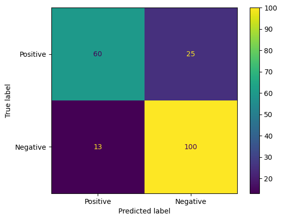
মডেল ভবিষ্যদ্বাণীগুলি মূল্যায়ন করার আরেকটি আকর্ষণীয় উপায় হল বিভ্রান্তি ম্যাট্রিক্স। একটি বিভ্রান্তি ম্যাট্রিক্স দৃশ্যত বিভিন্ন ধরণের ভবিষ্যদ্বাণী ত্রুটিগুলিকে চিত্রিত করবে।
from sklearn.metrics import confusion_matrix, ConfusionMatrixDisplay

cm = confusion_matrix(y_true, y_pred)
ConfusionMatrixDisplay(
    confusion_matrix=cm,
    display_labels=agile_classifier.labels,
).plot()
<sklearn.metrics._plot.confusion_matrix.ConfusionMatrixDisplay at 0x7eb7e2d29ab0>
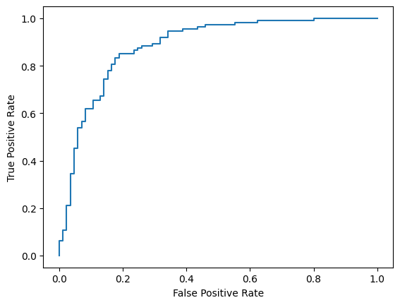
অবশেষে, আপনি বিভিন্ন স্কোরিং থ্রেশহোল্ড ব্যবহার করে সম্ভাব্য ভবিষ্যদ্বাণী ত্রুটির ধারণা পেতে ROC বক্ররেখাটিও দেখতে পারেন।
from sklearn.metrics import RocCurveDisplay, roc_curve

fpr, tpr, _ = roc_curve(y_true, y_prob, pos_label=1)
RocCurveDisplay(fpr=fpr, tpr=tpr).plot()
<sklearn.metrics._plot.roc_curve.RocCurveDisplay at 0x7eb4d130ef20>
পরিশিষ্ট
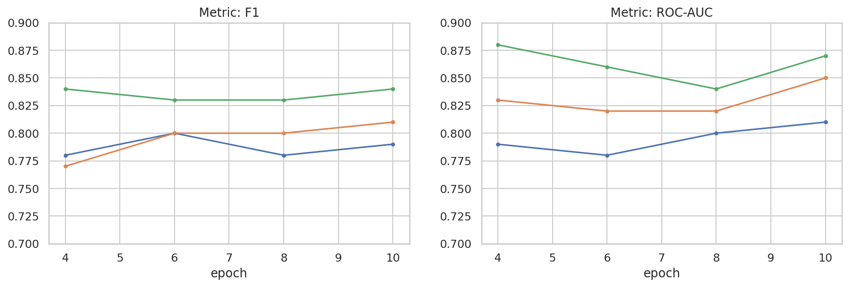
আমরা ডেটাসেটের আকার এবং কর্মক্ষমতার মধ্যে সম্পর্কের আরও ভাল ধারণা পেতে সাহায্য করার জন্য হাইপার-প্যারামিটার স্থানের কিছু মৌলিক অনুসন্ধান করেছি। নিম্নলিখিত প্লট দেখুন.
import matplotlib.pyplot as plt
import pandas as pd
import seaborn as sns

sns.set_theme(style="whitegrid")

results_f1 = pd.DataFrame([
    {'training_size': 800, 'epoch': 4, 'metric': 'f1', 'score': 0.84},
    {'training_size': 800, 'epoch': 6, 'metric': 'f1', 'score': 0.83},
    {'training_size': 800, 'epoch': 8, 'metric': 'f1', 'score': 0.83},
    {'training_size': 800, 'epoch': 10, 'metric': 'f1', 'score': 0.84},
    {'training_size': 400, 'epoch': 4, 'metric': 'f1', 'score': 0.77},
    {'training_size': 400, 'epoch': 6, 'metric': 'f1', 'score': 0.80},
    {'training_size': 400, 'epoch': 8, 'metric': 'f1', 'score': 0.80},
    {'training_size': 400, 'epoch': 10,'metric': 'f1', 'score': 0.81},
    {'training_size': 200, 'epoch': 4, 'metric': 'f1', 'score': 0.78},
    {'training_size': 200, 'epoch': 6, 'metric': 'f1', 'score': 0.80},
    {'training_size': 200, 'epoch': 8, 'metric': 'f1', 'score': 0.78},
    {'training_size': 200, 'epoch': 10, 'metric': 'f1', 'score': 0.79},
])

results_roc_auc = pd.DataFrame([
    {'training_size': 800, 'epoch': 4, 'metric': 'roc-auc', 'score': 0.88},
    {'training_size': 800, 'epoch': 6, 'metric': 'roc-auc', 'score': 0.86},
    {'training_size': 800, 'epoch': 8, 'metric': 'roc-auc', 'score': 0.84},
    {'training_size': 800, 'epoch': 10, 'metric': 'roc-auc', 'score': 0.87},
    {'training_size': 400, 'epoch': 4, 'metric': 'roc-auc', 'score': 0.83},
    {'training_size': 400, 'epoch': 6, 'metric': 'roc-auc', 'score': 0.82},
    {'training_size': 400, 'epoch': 8, 'metric': 'roc-auc', 'score': 0.82},
    {'training_size': 400, 'epoch': 10,'metric': 'roc-auc', 'score': 0.85},
    {'training_size': 200, 'epoch': 4, 'metric': 'roc-auc', 'score': 0.79},
    {'training_size': 200, 'epoch': 6, 'metric': 'roc-auc', 'score': 0.78},
    {'training_size': 200, 'epoch': 8, 'metric': 'roc-auc', 'score': 0.80},
    {'training_size': 200, 'epoch': 10, 'metric': 'roc-auc', 'score': 0.81},
])


plot_opts = dict(style='.-', ylim=(0.7, 0.9))
fig, (ax1, ax2) = plt.subplots(1, 2, figsize=(14, 4))
process_results_df = lambda df: df.set_index('epoch').groupby('training_size')['score']
process_results_df(results_f1).plot(title='Metric: F1', ax=ax1, **plot_opts)
process_results_df(results_roc_auc).plot(title='Metric: ROC-AUC', ax=ax2, **plot_opts)
fig.show()