|
|
|
 ดูซอร์สโค้ดใน GitHub ดูซอร์สโค้ดใน GitHub
|
|
โค้ดแล็บนี้แสดงวิธีสร้างตัวจัดประเภทข้อความที่กําหนดเองโดยใช้การปรับแต่งพารามิเตอร์ที่มีประสิทธิภาพ (PET) วิธีการ PET จะอัปเดตพารามิเตอร์เพียงไม่กี่รายการแทนการปรับแต่งโมเดลทั้งหมด ซึ่งทําให้การฝึกโมเดลค่อนข้างง่ายและรวดเร็ว นอกจากนี้ยังช่วยให้โมเดลเรียนรู้พฤติกรรมใหม่ๆ ได้ง่ายขึ้นด้วยข้อมูลการฝึกที่ไม่มากนัก วิธีการมีรายละเอียดอยู่ในบทความก้าวสู่ตัวแยกประเภทข้อความที่ยืดหยุ่นสำหรับทุกคน ซึ่งแสดงวิธีใช้เทคนิคเหล่านี้กับงานด้านความปลอดภัยที่หลากหลายและบรรลุประสิทธิภาพที่ล้ำสมัยด้วยตัวอย่างการฝึกเพียงไม่กี่ร้อยรายการ
โค้ดแล็บนี้ใช้วิธีการ PET ของ LoRA และ Gemma รุ่นที่เล็กกว่า (gemma_instruct_2b_en) เนื่องจากสามารถทำงานได้เร็วและมีประสิทธิภาพมากกว่า โคแลบนี้ครอบคลุมขั้นตอนการนำเข้าข้อมูล การจัดรูปแบบข้อมูลสำหรับ LLM การฝึกน้ำหนัก LoRA และการประเมินผลลัพธ์ โค้ดแล็บนี้ฝึกด้วยชุดข้อมูล ETHOS ซึ่งเป็นชุดข้อมูลสําหรับตรวจหาวาจาแสดงความเกลียดชังซึ่งเผยแพร่ต่อสาธารณะ โดยสร้างขึ้นจากความคิดเห็นใน YouTube และ Reddit
เมื่อฝึกด้วยตัวอย่างเพียง 200 รายการ (1/4 ของชุดข้อมูล) จะได้ F1: 0.80 และ ROC-AUC: 0.78 ซึ่งสูงกว่า SOTA ที่รายงานในตารางอันดับในปัจจุบันเล็กน้อย (ณ วันที่เขียน 15 ก.พ. 2024) เมื่อผ่านการฝึกด้วยตัวอย่างทั้งหมด 800 รายการ โมเดลนี้ได้รับคะแนน F1 เท่ากับ 83.74 และคะแนน ROC-AUC เท่ากับ 88.17 โดยทั่วไปแล้ว โมเดลขนาดใหญ่ เช่น gemma_instruct_7b_en จะมีประสิทธิภาพดีกว่า แต่ค่าใช้จ่ายในการฝึกและการดำเนินการก็จะสูงขึ้นด้วย
คำเตือน: เนื่องจากโค้ดแล็บนี้พัฒนาตัวแยกประเภทความปลอดภัยเพื่อตรวจหาวาจาสร้างความเกลียดชัง ตัวอย่างและการประเมินผลลัพธ์จึงมีภาษาที่รุนแรง
การติดตั้งและการตั้งค่า
สําหรับโค้ดแล็บนี้ คุณจะต้องมี keras (3) เวอร์ชันล่าสุด keras-nlp (0.8.0) และบัญชี Kaggle เพื่อดาวน์โหลดโมเดล Gemma
import kagglehub

kagglehub.login()
pip install -q -U keras-nlppip install -q -U keras
import os

os.environ["KERAS_BACKEND"] = "tensorflow"
โหลดชุดข้อมูล ETHOS
ในส่วนนี้ คุณจะโหลดชุดข้อมูลที่จะใช้ฝึกตัวแยกประเภท และประมวลผลข้อมูลเบื้องต้นเป็นชุดการฝึกและชุดทดสอบ คุณจะใช้ชุดข้อมูลการวิจัยยอดนิยมอย่าง ETHOS ซึ่งรวบรวมมาเพื่อตรวจหาวาจาสร้างความเกลียดชังบนโซเชียลมีเดีย ดูข้อมูลเพิ่มเติมเกี่ยวกับวิธีรวบรวมชุดข้อมูลได้ในบทความ ETHOS: ชุดข้อมูลการตรวจจับวาจาสร้างความเกลียดชังบนโลกออนไลน์
import pandas as pd

gh_root = 'https://raw.githubusercontent.com'
gh_repo = 'intelligence-csd-auth-gr/Ethos-Hate-Speech-Dataset'
gh_path = 'master/ethos/ethos_data/Ethos_Dataset_Binary.csv'
data_url = f'{gh_root}/{gh_repo}/{gh_path}'

df = pd.read_csv(data_url, delimiter=';')
df['hateful'] = (df['isHate'] >= df['isHate'].median()).astype(int)

# Shuffle the dataset.
df = df.sample(frac=1, random_state=32)

# Split into train and test.
df_train, df_test = df[:800],  df[800:]

# Display a sample of the data.
df.head(5)[['hateful', 'comment']]
ดาวน์โหลดและสร้างอินสแตนซ์โมเดล
คุณใช้โมเดล Gemma ได้หลายวิธีอย่างง่ายดายตามที่อธิบายไว้ในเอกสารประกอบ สิ่งที่ต้องทำใน Keras มีดังนี้
import keras
import keras_nlp

# For reproducibility purposes.
keras.utils.set_random_seed(1234)

# Download the model from Kaggle using Keras.
model = keras_nlp.models.GemmaCausalLM.from_preset('gemma_instruct_2b_en')

# Set the sequence length to a small enough value to fit in memory in Colab.
model.preprocessor.sequence_length = 128
model.generate('Question: what is the capital of France? ', max_length=32)
การเตรียมข้อความล่วงหน้าและโทเค็นตัวแบ่ง
คุณสามารถประมวลผลข้อความล่วงหน้าและใช้โทเค็นตัวคั่นเพื่อช่วยโมเดลให้เข้าใจความตั้งใจของเราได้ดียิ่งขึ้น วิธีนี้ช่วยลดโอกาสที่โมเดลจะสร้างข้อความที่ไม่ตรงกับรูปแบบที่คาดไว้ เช่น คุณอาจพยายามขอการจัดประเภทความรู้สึกจากโมเดลโดยเขียนพรอมต์เช่นนี้
Classify the following text into one of the following classes:[Positive,Negative]

Text: you look very nice today
Classification:
ในกรณีนี้ โมเดลอาจแสดงผลลัพธ์ที่คุณกำลังมองหาหรือไม่ก็ได้ เช่น หากข้อความมีอักขระบรรทัดใหม่ ก็อาจมีผลเสียต่อประสิทธิภาพของโมเดล แนวทางที่มีประสิทธิภาพมากขึ้นคือการใช้โทเค็นตัวคั่น จากนั้นพรอมต์จะเปลี่ยนเป็น
Classify the following text into one of the following classes:[Positive,Negative]
<separator>
Text: you look very nice today
<separator>
Prediction:
ซึ่งสามารถแยกออกมาได้โดยใช้ฟังก์ชันที่ประมวลผลข้อความล่วงหน้า ดังนี้
def preprocess_text(
    text: str,
    labels: list[str],
    instructions: str,
    separator: str,
) -> str:
  prompt = f'{instructions}:[{",".join(labels)}]'
  return separator.join([prompt, f'Text:{text}', 'Prediction:'])
ตอนนี้ หากคุณเรียกใช้ฟังก์ชันโดยใช้พรอมต์และข้อความเดียวกันกับก่อนหน้านี้ คุณควรได้ผลลัพธ์เดียวกัน ดังนี้
text = 'you look very nice today'

prompt = preprocess_text(
    text=text,
    labels=['Positive', 'Negative'],
    instructions='Classify the following text into one of the following classes',
    separator='\n<separator>\n',
)

print(prompt)
Classify the following text into one of the following classes:[Positive,Negative]
<separator>
Text:you look very nice today
<separator>
Prediction:
กระบวนการหลังการประมวลผลเอาต์พุต
เอาต์พุตของโมเดลคือโทเค็นที่มีความน่าจะเป็นต่างๆ โดยปกติแล้ว หากต้องการสร้างข้อความ คุณจะต้องเลือกโทเค็นที่เป็นไปได้มากที่สุด 2-3 รายการ แล้วสร้างประโยค ย่อหน้า หรือแม้แต่เอกสารทั้งฉบับ อย่างไรก็ตาม สําหรับวัตถุประสงค์การจัดประเภท สิ่งที่สําคัญจริงๆ คือการที่โมเดลเชื่อว่าPositiveมีแนวโน้มมากกว่าNegativeหรือในทางกลับกัน
เมื่อพิจารณาจากโมเดลที่คุณสร้างอินสแตนซ์ไว้ก่อนหน้านี้ นี่เป็นวิธีประมวลผลเอาต์พุตของโมเดลเป็นความน่าจะเป็นอิสระว่าโทเค็นถัดไปคือ Positive หรือ Negative ตามลำดับ
import numpy as np


def compute_output_probability(
    model: keras_nlp.models.GemmaCausalLM,
    prompt: str,
    target_classes: list[str],
) -> dict[str, float]:
  # Shorthands.
  preprocessor = model.preprocessor
  tokenizer = preprocessor.tokenizer

  # NOTE: If a token is not found, it will be considered same as "<unk>".
  token_unk = tokenizer.token_to_id('<unk>')

  # Identify the token indices, which is the same as the ID for this tokenizer.
  token_ids = [tokenizer.token_to_id(word) for word in target_classes]

  # Throw an error if one of the classes maps to a token outside the vocabulary.
  if any(token_id == token_unk for token_id in token_ids):
    raise ValueError('One of the target classes is not in the vocabulary.')

  # Preprocess the prompt in a single batch. This is done one sample at a time
  # for illustration purposes, but it would be more efficient to batch prompts.
  preprocessed = model.preprocessor.generate_preprocess([prompt])

  # Identify output token offset.
  padding_mask = preprocessed["padding_mask"]
  token_offset = keras.ops.sum(padding_mask) - 1

  # Score outputs, extract only the next token's logits.
  vocab_logits = model.score(
      token_ids=preprocessed["token_ids"],
      padding_mask=padding_mask,
  )[0][token_offset]

  # Compute the relative probability of each of the requested tokens.
  token_logits = [vocab_logits[ix] for ix in token_ids]
  logits_tensor = keras.ops.convert_to_tensor(token_logits)
  probabilities = keras.activations.softmax(logits_tensor)

  return dict(zip(target_classes, probabilities.numpy()))
คุณสามารถทดสอบฟังก์ชันดังกล่าวได้โดยเรียกใช้กับพรอมต์ที่คุณสร้างไว้ก่อนหน้านี้
compute_output_probability(
    model=model,
    prompt=prompt,
    target_classes=['Positive', 'Negative'],
)
{'Positive': 0.99994016, 'Negative': 5.984089e-05}
สรุปทั้งหมดเป็น Classfier
คุณสามารถรวมฟังก์ชันทั้งหมดที่เพิ่งสร้างขึ้นเป็นคลาสซิไฟเออร์แบบ sklearn รายการเดียวเพื่อให้ใช้งานได้ง่ายด้วยฟังก์ชันที่คุ้นเคย เช่น predict() และ predict_score()
import dataclasses


@dataclasses.dataclass(frozen=True)
class AgileClassifier:
  """Agile classifier to be wrapped around a LLM."""

  # The classes whose probability will be predicted.
  labels: tuple[str, ...]

  # Provide default instructions and control tokens, can be overridden by user.
  instructions: str = 'Classify the following text into one of the following classes'
  separator_token: str = '<separator>'
  end_of_text_token: str = '<eos>'

  def encode_for_prediction(self, x_text: str) -> str:
    return preprocess_text(
        text=x_text,
        labels=self.labels,
        instructions=self.instructions,
        separator=self.separator_token,
    )

  def encode_for_training(self, x_text: str, y: int) -> str:
    return ''.join([
        self.encode_for_prediction(x_text),
        self.labels[y],
        self.end_of_text_token,
    ])

  def predict_score(
      self,
      model: keras_nlp.models.GemmaCausalLM,
      x_text: str,
  ) -> list[float]:
    prompt = self.encode_for_prediction(x_text)
    token_probabilities = compute_output_probability(
        model=model,
        prompt=prompt,
        target_classes=self.labels,
    )
    return [token_probabilities[token] for token in self.labels]

  def predict(
      self,
      model: keras_nlp.models.GemmaCausalLM,
      x_eval: str,
  ) -> int:
    return np.argmax(self.predict_score(model, x_eval))

agile_classifier = AgileClassifier(labels=('Positive', 'Negative'))
การปรับแต่งโมเดล
LoRA ย่อมาจาก Low-Rank Adaptation ซึ่งเป็นเทคนิคการปรับแต่งที่สามารถนำไปใช้ปรับแต่งโมเดลภาษาขนาดใหญ่ได้อย่างมีประสิทธิภาพ อ่านเพิ่มเติมเกี่ยวกับเรื่องนี้ได้ในบทความLoRA: การปรับเปลี่ยนโมเดลภาษาขนาดใหญ่แบบ Low-Rank
การใช้งาน Gemma ใน Keras มีenable_lora()เมธอดที่คุณใช้เพื่อปรับแต่งได้ ดังนี้
# Enable LoRA for the model and set the LoRA rank to 4.
model.backbone.enable_lora(rank=4)
หลังจากเปิดใช้ LoRA แล้ว คุณสามารถเริ่มกระบวนการปรับแต่งได้ การดำเนินการนี้จะใช้เวลาประมาณ 5 นาทีต่อแต่ละยุคใน Colab
import tensorflow as tf

# Create dataset with preprocessed text + labels.
map_fn = lambda x: agile_classifier.encode_for_training(*x)
x_train = list(map(map_fn, df_train[['comment', 'hateful']].values))
ds_train = tf.data.Dataset.from_tensor_slices(x_train).batch(2)

# Compile the model using the Adam optimizer and appropriate loss function.
model.compile(
    loss=keras.losses.SparseCategoricalCrossentropy(from_logits=True),
    optimizer=keras.optimizers.Adam(learning_rate=0.0005),
    weighted_metrics=[keras.metrics.SparseCategoricalAccuracy()],
)

# Begin training.
model.fit(ds_train, epochs=4)
Epoch 1/4
400/400 ━━━━━━━━━━━━━━━━━━━━ 354s 703ms/step - loss: 1.1365 - sparse_categorical_accuracy: 0.5874
Epoch 2/4
400/400 ━━━━━━━━━━━━━━━━━━━━ 338s 716ms/step - loss: 0.7579 - sparse_categorical_accuracy: 0.6662
Epoch 3/4
400/400 ━━━━━━━━━━━━━━━━━━━━ 324s 721ms/step - loss: 0.6818 - sparse_categorical_accuracy: 0.6894
Epoch 4/4
400/400 ━━━━━━━━━━━━━━━━━━━━ 323s 725ms/step - loss: 0.5922 - sparse_categorical_accuracy: 0.7220
<keras.src.callbacks.history.History at 0x7eb7e369c490>
การฝึกอบรมในจำนวนรอบมากขึ้นจะทําให้เกิดความแม่นยำสูงขึ้น จนกว่าจะเกิดภาวะการเรียนรู้มากเกินไป
ตรวจสอบผลลัพธ์
ตอนนี้คุณตรวจสอบเอาต์พุตของตัวแยกประเภทแบบยืดหยุ่นที่เพิ่งฝึกแล้วได้ โค้ดนี้จะแสดงผลคะแนนชั้นเรียนที่คาดการณ์จากข้อความ
text = 'you look really nice today'
scores = agile_classifier.predict_score(model, text)
dict(zip(agile_classifier.labels, scores))
{'Positive': 0.99899644, 'Negative': 0.0010035498}
การประเมินโมเดล
สุดท้าย คุณประเมินประสิทธิภาพของโมเดลโดยใช้เมตริกทั่วไป 2 รายการ ได้แก่ คะแนน F1 และ AUC-ROC คะแนน F1 จะบันทึกข้อผิดพลาดเชิงลบและผลบวกลวงโดยประเมินค่าเฉลี่ยฮาร์โมนิกของความแม่นยำและความแม่นยำสัมพัทธ์ที่เกณฑ์การจัดประเภทหนึ่งๆ ส่วน AUC-ROC แสดงให้เห็นถึงการตัดกันระหว่างอัตราผลบวกจริงกับอัตราผลบวกลวงในเกณฑ์ต่างๆ และคำนวณพื้นที่ใต้เส้นโค้งนี้
y_true = df_test['hateful'].values
# Compute the scores (aka probabilities) for each of the labels.
y_score = [agile_classifier.predict_score(model, x) for x in df_test['comment']]
# The label with highest score is considered the predicted class.
y_pred = np.argmax(y_score, axis=1)
# Extract the probability of a comment being considered hateful.
y_prob = [x[agile_classifier.labels.index('Negative')] for x in y_score]
from sklearn.metrics import f1_score, roc_auc_score

print(f'F1: {f1_score(y_true, y_pred):.2f}')
print(f'AUC-ROC: {roc_auc_score(y_true, y_prob):.2f}')
F1: 0.84
AUC-ROC: 0.88
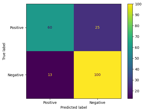
อีกวิธีที่น่าสนใจในการประเมินการคาดการณ์ของโมเดลคือเมทริกซ์ความสับสน ตารางความสับสนจะแสดงข้อผิดพลาดในการคาดการณ์ประเภทต่างๆ เป็นภาพ
from sklearn.metrics import confusion_matrix, ConfusionMatrixDisplay

cm = confusion_matrix(y_true, y_pred)
ConfusionMatrixDisplay(
    confusion_matrix=cm,
    display_labels=agile_classifier.labels,
).plot()
<sklearn.metrics._plot.confusion_matrix.ConfusionMatrixDisplay at 0x7eb7e2d29ab0>
สุดท้าย คุณยังดูเส้นโค้ง ROC เพื่อประเมินข้อผิดพลาดในการคาดการณ์ที่อาจเกิดขึ้นเมื่อใช้เกณฑ์การให้คะแนนที่แตกต่างกันได้ด้วย
from sklearn.metrics import RocCurveDisplay, roc_curve

fpr, tpr, _ = roc_curve(y_true, y_prob, pos_label=1)
RocCurveDisplay(fpr=fpr, tpr=tpr).plot()
<sklearn.metrics._plot.roc_curve.RocCurveDisplay at 0x7eb4d130ef20>

ภาคผนวก
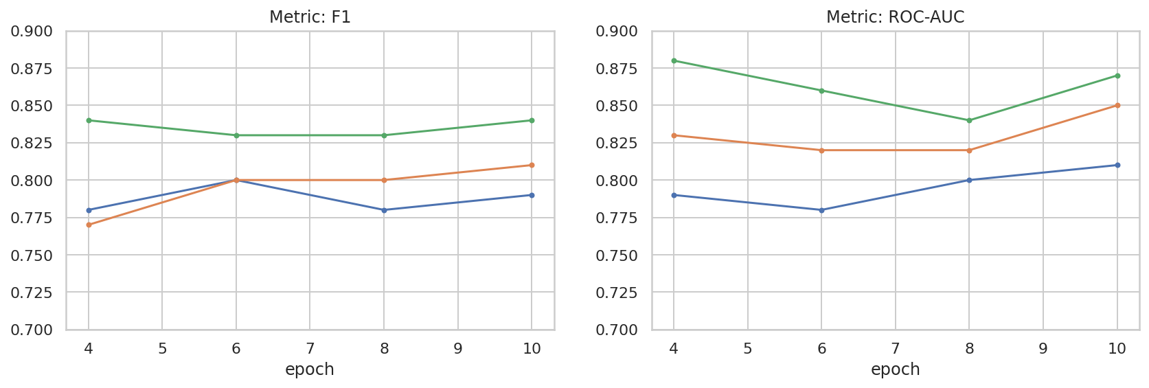
เราได้ทำการสำรวจเบื้องต้นเกี่ยวกับพื้นที่พารามิเตอร์ไฮเปอร์เพื่อช่วยให้คุณเข้าใจความสัมพันธ์ระหว่างขนาดชุดข้อมูลกับประสิทธิภาพได้ดียิ่งขึ้น ดูผังต่อไปนี้
import matplotlib.pyplot as plt
import pandas as pd
import seaborn as sns

sns.set_theme(style="whitegrid")

results_f1 = pd.DataFrame([
    {'training_size': 800, 'epoch': 4, 'metric': 'f1', 'score': 0.84},
    {'training_size': 800, 'epoch': 6, 'metric': 'f1', 'score': 0.83},
    {'training_size': 800, 'epoch': 8, 'metric': 'f1', 'score': 0.83},
    {'training_size': 800, 'epoch': 10, 'metric': 'f1', 'score': 0.84},
    {'training_size': 400, 'epoch': 4, 'metric': 'f1', 'score': 0.77},
    {'training_size': 400, 'epoch': 6, 'metric': 'f1', 'score': 0.80},
    {'training_size': 400, 'epoch': 8, 'metric': 'f1', 'score': 0.80},
    {'training_size': 400, 'epoch': 10,'metric': 'f1', 'score': 0.81},
    {'training_size': 200, 'epoch': 4, 'metric': 'f1', 'score': 0.78},
    {'training_size': 200, 'epoch': 6, 'metric': 'f1', 'score': 0.80},
    {'training_size': 200, 'epoch': 8, 'metric': 'f1', 'score': 0.78},
    {'training_size': 200, 'epoch': 10, 'metric': 'f1', 'score': 0.79},
])

results_roc_auc = pd.DataFrame([
    {'training_size': 800, 'epoch': 4, 'metric': 'roc-auc', 'score': 0.88},
    {'training_size': 800, 'epoch': 6, 'metric': 'roc-auc', 'score': 0.86},
    {'training_size': 800, 'epoch': 8, 'metric': 'roc-auc', 'score': 0.84},
    {'training_size': 800, 'epoch': 10, 'metric': 'roc-auc', 'score': 0.87},
    {'training_size': 400, 'epoch': 4, 'metric': 'roc-auc', 'score': 0.83},
    {'training_size': 400, 'epoch': 6, 'metric': 'roc-auc', 'score': 0.82},
    {'training_size': 400, 'epoch': 8, 'metric': 'roc-auc', 'score': 0.82},
    {'training_size': 400, 'epoch': 10,'metric': 'roc-auc', 'score': 0.85},
    {'training_size': 200, 'epoch': 4, 'metric': 'roc-auc', 'score': 0.79},
    {'training_size': 200, 'epoch': 6, 'metric': 'roc-auc', 'score': 0.78},
    {'training_size': 200, 'epoch': 8, 'metric': 'roc-auc', 'score': 0.80},
    {'training_size': 200, 'epoch': 10, 'metric': 'roc-auc', 'score': 0.81},
])


plot_opts = dict(style='.-', ylim=(0.7, 0.9))
fig, (ax1, ax2) = plt.subplots(1, 2, figsize=(14, 4))
process_results_df = lambda df: df.set_index('epoch').groupby('training_size')['score']
process_results_df(results_f1).plot(title='Metric: F1', ax=ax1, **plot_opts)
process_results_df(results_roc_auc).plot(title='Metric: ROC-AUC', ax=ax2, **plot_opts)
fig.show()