
|
|
|
 GitHub のノートブックを表示 GitHub のノートブックを表示
|
概要
このチュートリアルでは、Gemini API のエンベディングを使用してデータセット内の潜在的な外れ値を検出する方法について説明します。20 の Newsgroup データセットのサブセットを t-SNE を使用して可視化し、各カテゴリ クラスタの中心点から特定の半径の外側にある外れ値を検出します。
Gemini API で生成されたエンベディングの使用を開始する方法について詳しくは、Python クイックスタートをご覧ください。
前提条件
このクイックスタートは Google Colab で実行できます。
このクイックスタートを独自の開発環境で完了するには、環境が次の要件を満たしていることを確認してください。
- Python 3.9 以降
- ノートブックを実行するための
jupyterのインストール。
セットアップ
まず、Gemini API Python ライブラリをダウンロードしてインストールします。
pip install -U -q google.generativeai
import re
import tqdm
import numpy as np
import pandas as pd
import matplotlib.pyplot as plt
import seaborn as sns

import google.generativeai as genai

# Used to securely store your API key
from google.colab import userdata

from sklearn.datasets import fetch_20newsgroups
from sklearn.manifold import TSNE
API キーを取得
Gemini API を使用するには、まず API キーを取得する必要があります。キーをまだ作成していない場合は、Google AI Studio でワンクリックで作成できます。
Colab で、シークレット マネージャーに鍵を追加する「メンズ」を使用します。をクリックします。API_KEY という名前を付けます。
API キーを取得したら、SDK に渡します。作成する方法は次の 2 つです。
- 鍵を
GOOGLE_API_KEY環境変数に設定します(SDK はそこから自動的に取得します)。 - 鍵を
genai.configure(api_key=...)に渡す
genai.configure(api_key=GOOGLE_API_KEY)
for m in genai.list_models():
  if 'embedContent' in m.supported_generation_methods:
    print(m.name)
models/embedding-001
models/embedding-001
データセットを準備する
20 Newsgroups Text Dataset には、トレーニング セットとテストセットに分けられた 20 トピックに関する 18,000 件のニュースグループ投稿が含まれています。トレーニング データセットとテスト データセットの分割は、特定の日付の前後に投稿されたメッセージに基づいて行われます。このチュートリアルでは、トレーニング サブセットを使用します。
newsgroups_train = fetch_20newsgroups(subset='train')

# View list of class names for dataset
newsgroups_train.target_names
['alt.atheism',
 'comp.graphics',
 'comp.os.ms-windows.misc',
 'comp.sys.ibm.pc.hardware',
 'comp.sys.mac.hardware',
 'comp.windows.x',
 'misc.forsale',
 'rec.autos',
 'rec.motorcycles',
 'rec.sport.baseball',
 'rec.sport.hockey',
 'sci.crypt',
 'sci.electronics',
 'sci.med',
 'sci.space',
 'soc.religion.christian',
 'talk.politics.guns',
 'talk.politics.mideast',
 'talk.politics.misc',
 'talk.religion.misc']
こちらがトレーニング セットの最初の例です。
idx = newsgroups_train.data[0].index('Lines')
print(newsgroups_train.data[0][idx:])
Lines: 15

 I was wondering if anyone out there could enlighten me on this car I saw
the other day. It was a 2-door sports car, looked to be from the late 60s/
early 70s. It was called a Bricklin. The doors were really small. In addition,
the front bumper was separate from the rest of the body. This is
all I know. If anyone can tellme a model name, engine specs, years
of production, where this car is made, history, or whatever info you
have on this funky looking car, please e-mail.

Thanks,

- IL
   ---- brought to you by your neighborhood Lerxst ----
# Apply functions to remove names, emails, and extraneous words from data points in newsgroups.data
newsgroups_train.data = [re.sub(r'[\w\.-]+@[\w\.-]+', '', d) for d in newsgroups_train.data] # Remove email
newsgroups_train.data = [re.sub(r"\([^()]*\)", "", d) for d in newsgroups_train.data] # Remove names
newsgroups_train.data = [d.replace("From: ", "") for d in newsgroups_train.data] # Remove "From: "
newsgroups_train.data = [d.replace("\nSubject: ", "") for d in newsgroups_train.data] # Remove "\nSubject: "

# Cut off each text entry after 5,000 characters
newsgroups_train.data = [d[0:5000] if len(d) > 5000 else d for d in newsgroups_train.data]
# Put training points into a dataframe
df_train = pd.DataFrame(newsgroups_train.data, columns=['Text'])
df_train['Label'] = newsgroups_train.target
# Match label to target name index
df_train['Class Name'] = df_train['Label'].map(newsgroups_train.target_names.__getitem__)

df_train
次に、トレーニング データセット内の 150 個のデータポイントを取得し、いくつかのカテゴリを選択して、一部のデータをサンプリングします。このチュートリアルでは、科学のカテゴリを使用します。
# Take a sample of each label category from df_train
SAMPLE_SIZE = 150
df_train = (df_train.groupby('Label', as_index = False)
                    .apply(lambda x: x.sample(SAMPLE_SIZE))
                    .reset_index(drop=True))

# Choose categories about science
df_train = df_train[df_train['Class Name'].str.contains('sci')]

# Reset the index
df_train = df_train.reset_index()
df_train
df_train['Class Name'].value_counts()
sci.crypt          150
sci.electronics    150
sci.med            150
sci.space          150
Name: Class Name, dtype: int64
エンベディングを作成する
このセクションでは、Gemini API のエンベディングを使用して、データフレーム内のさまざまなテキストのエンベディングを生成する方法について説明します。
モデル embedding-001 によるエンべディングの API の変更
新しいエンベディング モデル embedding-001 には、新しいタスクタイプ パラメータとオプションのタイトルがあります(task_type=RETRIEVAL_DOCUMENT の場合のみ有効です)。
これらの新しいパラメータは、最新のエンベディング モデルにのみ適用されます。タスクの種類は次のとおりです。
| タスクの種類 | 説明 |
|---|---|
| RETRIEVAL_QUERY | 指定したテキストが検索 / 取得設定のクエリであることを指定します。 |
| RETRIEVAL_DOCUMENT | 指定したテキストが検索 / 取得設定のドキュメントであることを指定します。 |
| SEMANTIC_SIMILARITY | 指定したテキストが意味論的テキスト類似性(STS)で使用されることを指定します。 |
| 分類 | エンベディングを分類に使用することを指定します。 |
| クラスタリング | エンベディングをクラスタリングに使用することを指定します。 |
from tqdm.auto import tqdm
tqdm.pandas()

from google.api_core import retry

def make_embed_text_fn(model):

  @retry.Retry(timeout=300.0)
  def embed_fn(text: str) -> list[float]:
    # Set the task_type to CLUSTERING.
    embedding = genai.embed_content(model=model,
                                    content=text,
                                    task_type="clustering")['embedding']
    return np.array(embedding)

  return embed_fn

def create_embeddings(df):
  model = 'models/embedding-001'
  df['Embeddings'] = df['Text'].progress_apply(make_embed_text_fn(model))
  return df

df_train = create_embeddings(df_train)
df_train.drop('index', axis=1, inplace=True)
0%| | 0/600 [00:00<?, ?it/s]
次元数の削減
ドキュメントのエンベディング ベクトルの次元は 768 です。埋め込みドキュメントがどのようにグループ化されているかを可視化するには、エンベディングを 2D または 3D 空間でしか可視化できないため、次元数を削減する必要があります。文脈的に類似したドキュメントは、類似していないドキュメントとは対照的に、スペース内で近くする必要があります。
len(df_train['Embeddings'][0])
768
# Convert df_train['Embeddings'] Pandas series to a np.array of float32
X = np.array(df_train['Embeddings'].to_list(), dtype=np.float32)
X.shape
(600, 768)
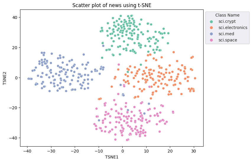
t 分散確率近傍エンベディング(t-SNE)アプローチを適用して、次元数を削減します。この手法では、次元の数を減らしながら、クラスタ(近接するポイント同士の距離を保ちます)を維持できます。元のデータについて、他のデータポイントが「近傍」である分布を構築しようとする(例: 意味が似ている)。次に、目的関数を最適化して、可視化において同様の分布を維持します。
tsne = TSNE(random_state=0, n_iter=1000)
tsne_results = tsne.fit_transform(X)
df_tsne = pd.DataFrame(tsne_results, columns=['TSNE1', 'TSNE2'])
df_tsne['Class Name'] = df_train['Class Name'] # Add labels column from df_train to df_tsne
df_tsne
fig, ax = plt.subplots(figsize=(8,6)) # Set figsize
sns.set_style('darkgrid', {"grid.color": ".6", "grid.linestyle": ":"})
sns.scatterplot(data=df_tsne, x='TSNE1', y='TSNE2', hue='Class Name', palette='Set2')
sns.move_legend(ax, "upper left", bbox_to_anchor=(1, 1))
plt.title('Scatter plot of news using t-SNE')
plt.xlabel('TSNE1')
plt.ylabel('TSNE2');
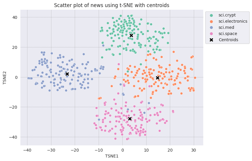
外れ値検出
どのポイントが異常かを判断するには、どのポイントが外れ値かを判断します。まず、クラスタの中心を表すセントロイド(位置)を見つけ、その距離から外れ値となる点を特定します。
まず、各カテゴリのセントロイドを取得します。
def get_centroids(df_tsne):
  # Get the centroid of each cluster
  centroids = df_tsne.groupby('Class Name').mean()
  return centroids

centroids = get_centroids(df_tsne)
centroids
def get_embedding_centroids(df):
  emb_centroids = dict()
  grouped = df.groupby('Class Name')
  for c in grouped.groups:
    sub_df = grouped.get_group(c)
    # Get the centroid value of dimension 768
    emb_centroids[c] = np.mean(sub_df['Embeddings'], axis=0)

  return emb_centroids
emb_c = get_embedding_centroids(df_train)
見つけた各重心を残りの点に対してプロットします。
# Plot the centroids against the cluster
fig, ax = plt.subplots(figsize=(8,6)) # Set figsize
sns.set_style('darkgrid', {"grid.color": ".6", "grid.linestyle": ":"})
sns.scatterplot(data=df_tsne, x='TSNE1', y='TSNE2', hue='Class Name', palette='Set2');
sns.scatterplot(data=centroids, x='TSNE1', y='TSNE2', color="black", marker='X', s=100, label='Centroids')
sns.move_legend(ax, "upper left", bbox_to_anchor=(1, 1))
plt.title('Scatter plot of news using t-SNE with centroids')
plt.xlabel('TSNE1')
plt.ylabel('TSNE2');
半径を選択します。そのカテゴリのセントロイドからこの境界を超えるものは、外れ値とみなされます。
def calculate_euclidean_distance(p1, p2):
  return np.sqrt(np.sum(np.square(p1 - p2)))

def detect_outlier(df, emb_centroids, radius):
  for idx, row in df.iterrows():
    class_name = row['Class Name'] # Get class name of row
    # Compare centroid distances
    dist = calculate_euclidean_distance(row['Embeddings'],
                                        emb_centroids[class_name])
    df.at[idx, 'Outlier'] = dist > radius

  return len(df[df['Outlier'] == True])
range_ = np.arange(0.3, 0.75, 0.02).round(decimals=2).tolist()
num_outliers = []
for i in range_:
  num_outliers.append(detect_outlier(df_train, emb_c, i))
# Plot range_ and num_outliers
fig = plt.figure(figsize = (14, 8))
plt.rcParams.update({'font.size': 12})
plt.bar(list(map(str, range_)), num_outliers)
plt.title("Number of outliers vs. distance of points from centroid")
plt.xlabel("Distance")
plt.ylabel("Number of outliers")
for i in range(len(range_)):
  plt.text(i, num_outliers[i], num_outliers[i], ha = 'center')

plt.show()
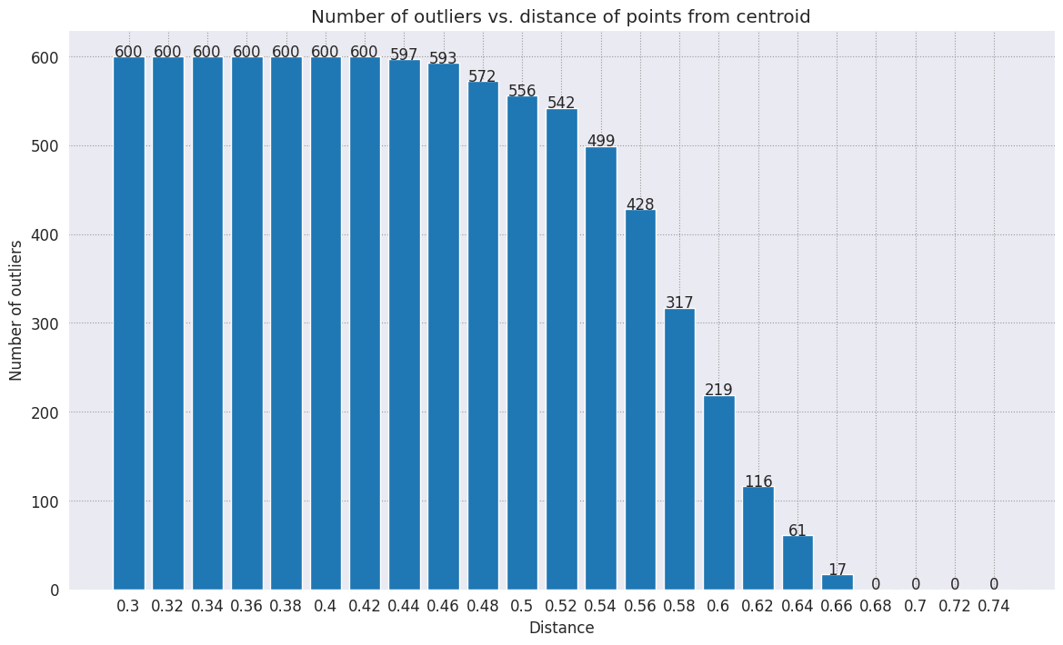
異常検出機能に求める感度に応じて、使用する半径を選択できます。現時点では 0.62 が使用されますが、この値は変更できます。
# View the points that are outliers
RADIUS = 0.62
detect_outlier(df_train, emb_c, RADIUS)
df_outliers = df_train[df_train['Outlier'] == True]
df_outliers.head()
# Use the index to map the outlier points back to the projected TSNE points
outliers_projected = df_tsne.loc[df_outliers['Outlier'].index]
外れ値をプロットし、透明な赤色で示します。
fig, ax = plt.subplots(figsize=(8,6)) # Set figsize
plt.rcParams.update({'font.size': 10})
sns.set_style('darkgrid', {"grid.color": ".6", "grid.linestyle": ":"})
sns.scatterplot(data=df_tsne, x='TSNE1', y='TSNE2', hue='Class Name', palette='Set2');
sns.scatterplot(data=centroids, x='TSNE1', y='TSNE2', color="black", marker='X', s=100, label='Centroids')
# Draw a red circle around the outliers
sns.scatterplot(data=outliers_projected, x='TSNE1', y='TSNE2', color='red', marker='o', alpha=0.5, s=90, label='Outliers')
sns.move_legend(ax, "upper left", bbox_to_anchor=(1, 1))
plt.title('Scatter plot of news with outliers projected with t-SNE')
plt.xlabel('TSNE1')
plt.ylabel('TSNE2');
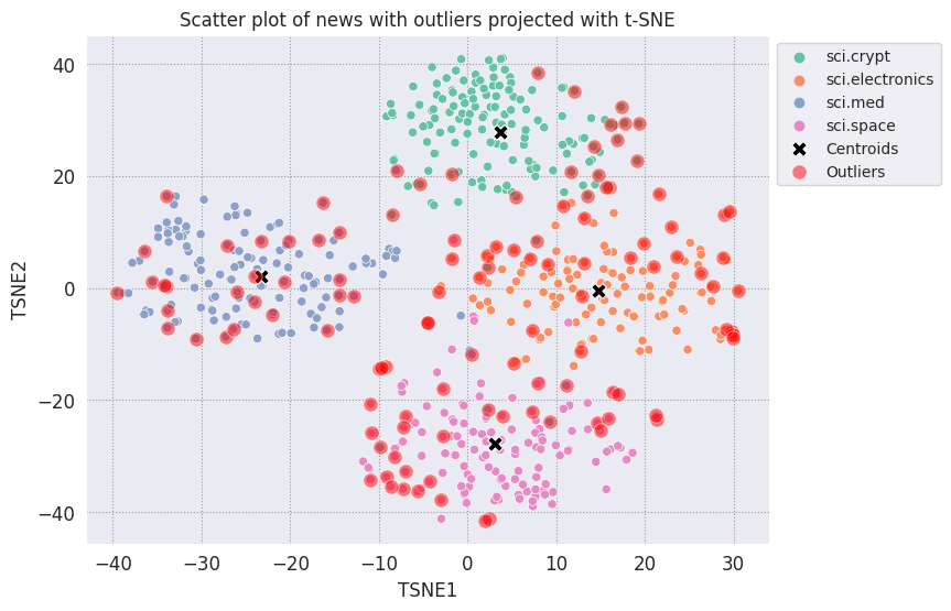
データファムのインデックス値を使用して、各カテゴリの外れ値の例をいくつか出力します。ここでは、各カテゴリの最初のデータポイントが出力されます。各カテゴリの他のポイントを調べて、外れ値や異常とみなされるデータを確認します。
sci_crypt_outliers = df_outliers[df_outliers['Class Name'] == 'sci.crypt']
print(sci_crypt_outliers['Text'].iloc[0])
Re: Source of random bits on a Unix workstation
Lines: 44
Nntp-Posting-Host: sandstorm

>>For your application, what you can do is to encrypt the real-time clock
>>value with a secret key.

Well, almost.... If I only had to solve the problem for myself, and were
willing to have to type in a second password  whenever I
logged in, it could work. However, I'm trying to create a solution that
anyone can use, and which, once installed, is just as effortless to start up
as the non-solution of just using xhost to control access. I've got
religeous problems with storing secret keys on multiuser computers.

>For a good discussion of cryptographically "good" random number
>generators, check out the draft-ietf-security-randomness-00.txt
>Internet Draft, available at your local friendly internet drafts
>repository.

Thanks for the pointer! It was good reading, and I liked the idea of using
several unrelated sources with a strong mixing function. However, unless I
missed something, the only source they suggested
that seems available, and unguessable by an intruder, when a Unix is
fresh-booted, is I/O buffers related to network traffic. I believe my
solution basically uses that strategy, without requiring me to reach into
the kernel.

>A reasonably source of randomness is the output of a cryptographic
>hash function , when fed with a large amount of
>more-or-less random data. For example, running MD5 on /dev/mem is a
>slow, but random enough, source of random bits; there are bound to be
>128 bits of entropy in the tens  of megabytes of data in
>a modern workstation's memory, as a fair amount of them are system
>timers, i/o buffers, etc.

I heard about this solution, and it sounded good. Then I heard that folks
were experiencing times of 30-60 seconds to run this, on
reasonably-configured workstations. I'm not willing to add that much delay
to someone's login process. My approach  takes
a second or two to run. I'm considering writing the be-all and end-all of
solutions, that launches the MD5, and simultaneously tries to suck bits off
the net, and if the net should be sitting __SO__ idle that it can't get 10K
after compression before MD5 finishes, use the MD5. This way I could have
guaranteed good bits, and a deterministic upper bound on login time, and
still have the common case of login take only a couple of extra seconds.

-Bennett
sci_elec_outliers = df_outliers[df_outliers['Class Name'] == 'sci.electronics']
print(sci_elec_outliers['Text'].iloc[0])
Re: Laser vs Bubblejet?
Reply-To:
Distribution: world
X-Mailer: cppnews \\(Revision: 1.20 \\)
Organization: null
Lines: 53

Here is a different viewpoint.

> FYI:  The actual horizontal dot placement resoution of an HP
> deskjet is 1/600th inch.  The electronics and dynamics of the ink
> cartridge, however, limit you to generating dots at 300 per inch.
> On almost any paper, the ink wicks more than 1/300th inch anyway.
>
> The method of depositing and fusing toner of a laster printer
> results in much less spread than ink drop technology.

In practice there is little difference in quality but more care is needed
with inkjet because smudges etc. can happen.

> It doesn't take much investigation to see that the mechanical and
> electronic complement of a laser printer is more complex than
> inexpensive ink jet printers.  Recall also that laser printers
> offer a much higher throughput:  10 ppm for a laser versus about 1
> ppm for an ink jet printer.

A cheap laser printer does not manage that sort of throughput and on top of
that how long does the _first_ sheet take to print? Inkjets are faster than
you say and in both cases the computer often has trouble keeping up with the
printer.

A sage said to me: "Do you want one copy or lots of copies?", "One",
"Inkjet".

> Something else to think about is the cost of consumables over the
> life of the printer.  A 3000 page yield toner cartridge is about
> $US 75-80 at discount while HP high capacity
> cartridges are about $US 22 at discount.  It could be that over the
> life cycle of the printer that consumables for laser printers are
> less than ink jet printers.  It is getting progressively closer
> between the two technologies.  Laser printers are usually desinged
> for higher duty cycles in pages per month and longer product
> replacement cycles.

Paper cost is the same and both can use refills. Long term the laserprinter
will need some expensive replacement parts  and on top of that
are the amortisation costs which favour the lowest purchase cost printer.

HP inkjets understand PCL so in many cases a laserjet driver will work if the
software package has no inkjet driver.

There is one wild difference between the two printers: a laserprinter is a
page printer whilst an inkjet is a line printer. This means that a
laserprinter can rotate graphic images whilst an inkjet cannot. Few drivers
actually use this facility.


  TC.
    E-mail:  or
sci_med_outliers = df_outliers[df_outliers['Class Name'] == 'sci.med']
print(sci_med_outliers['Text'].iloc[0])
Re: THE BACK MACHINE - Update
Organization: University of Nebraska--Lincoln
Lines: 15
Distribution: na
NNTP-Posting-Host: unlinfo.unl.edu

   I have a BACK MACHINE and have had one since January.  While I have not
found it to be a panacea for my back pain, I think it has helped somewhat.
It MAINLY acts to stretch muscles in the back and prevent spasms associated
with pain.  I am taking less pain medication than I was previously.
   The folks at BACK TECHNOLOGIES are VERY reluctant to honor their return
policy.  They extended my "warranty" period rather than allow me to return
the machine when, after the first month or so, I was not thrilled with it.
They encouraged me to continue to use it, abeit less vigourously.
   Like I said, I can't say it is a cure-all, but it keeps me stretched out
and I am in less pain.
--
***********************************************************************
Dale M. Webb, DVM, PhD           *  97% of the body is water.  The
Veterinary Diagnostic Center     *  other 3% keeps you from drowning.
University of Nebraska, Lincoln  *
sci_space_outliers = df_outliers[df_outliers['Class Name'] == 'sci.space']
print(sci_space_outliers['Text'].iloc[0])
MACH 25 landing site bases?
Article-I.D.: aurora.1993Apr5.193829.1
Organization: University of Alaska Fairbanks
Lines: 7
Nntp-Posting-Host: acad3.alaska.edu

The supersonic booms hear a few months ago over I belive San Fran, heading east
of what I heard, some new super speed Mach 25 aircraft?? What military based
int he direction of flight are there that could handle a Mach 25aircraft on its
landing decent?? Odd question??

==
Michael Adams,  -- I'm not high, just jacked
次のステップ
これで、エンベディングを使用して異常検出機能を作成できました。独自のテキストデータを使用してエンベディングとして可視化し、外れ値を検出できるように境界を選択します。可視化のステップを完了するために、次元数を削減できます。t-SNE は入力のクラスタリングに適していますが、収束に時間がかかる場合や、局所的な最小値で停止する場合があります。この問題が発生した場合は、主成分分析(PCA)という手法も検討できます。
エンベディングの使用方法について詳しくは、以下のチュートリアルをご覧ください。