Gemini 1.5 Flash 가격 인하, 모든 개발자를 위한 액세스 세부 조정 등 자세히 알아보기

이 페이지는 Cloud Translation API를 통해 번역되었습니다.

임베딩을 사용한 이상 감지

ai.google.dev에서 보기

Colab 노트북 사용해 보기

GitHub에서 노트북 보기

개요

이 튜토리얼에서는 Gemini API의 임베딩을 사용하여 데이터 세트에서 잠재적인 이상점을 감지하는 방법을 보여줍니다. t-SNE를 사용하여 20개 뉴스그룹 데이터 세트의 하위 집합을 시각화하고 각 범주형 클러스터 중심점의 특정 반경을 벗어나는 이상점을 감지합니다.

Gemini API에서 생성된 임베딩을 시작하는 방법에 대한 자세한 내용은 Python 빠른 시작을 확인하세요.

기본 요건

이 빠른 시작은 Google Colab에서 실행할 수 있습니다.

자체 개발 환경에서 이 빠른 시작을 완료하려면 환경이 다음 요구사항을 충족하는지 확인하세요.

Python 3.9 이상
노트북 실행을 위한 jupyter 설치

설정

먼저 Gemini API Python 라이브러리를 다운로드하고 설치합니다.

pip install -U -q google.generativeai

import re
import tqdm
import numpy as np
import pandas as pd
import matplotlib.pyplot as plt
import seaborn as sns

import google.generativeai as genai

# Used to securely store your API key
from google.colab import userdata

from sklearn.datasets import fetch_20newsgroups
from sklearn.manifold import TSNE

API 키 가져오기

Gemini API를 사용하려면 먼저 API 키를 받아야 합니다. 아직 키가 없다면 Google AI Studio에서 클릭 한 번으로 키를 만듭니다.

API 키 가져오기

Colab에서 'recommended' 아래의 보안 비밀 관리자에 키를 추가하세요. 왼쪽 패널에 표시됩니다. 이름을 API_KEY로 지정합니다.

API 키를 확보하면 이를 SDK에 전달합니다. 여기에는 두 가지 방법이 있습니다.

키를 GOOGLE_API_KEY 환경 변수에 입력합니다. SDK가 이 환경 변수에서 키를 자동으로 선택합니다.
키를 genai.configure(api_key=...)에 전달

를 통해 개인정보처리방침을 정의할 수 있습니다.

genai.configure(api_key=GOOGLE_API_KEY)

for m in genai.list_models():
  if 'embedContent' in m.supported_generation_methods:
    print(m.name)

models/embedding-001
models/embedding-001

데이터 세트 준비

20 Newsgroups Text Dataset에는 학습 세트와 테스트 세트로 나뉘어 20개 주제에 관한 18,000개의 뉴스그룹 게시물이 포함되어 있습니다. 학습 데이터 세트와 테스트 데이터 세트 간의 분할은 특정 날짜 전후에 게시된 메시지를 기준으로 합니다. 이 튜토리얼에서는 학습 하위 집합을 사용합니다.

newsgroups_train = fetch_20newsgroups(subset='train')

# View list of class names for dataset
newsgroups_train.target_names

['alt.atheism',
 'comp.graphics',
 'comp.os.ms-windows.misc',
 'comp.sys.ibm.pc.hardware',
 'comp.sys.mac.hardware',
 'comp.windows.x',
 'misc.forsale',
 'rec.autos',
 'rec.motorcycles',
 'rec.sport.baseball',
 'rec.sport.hockey',
 'sci.crypt',
 'sci.electronics',
 'sci.med',
 'sci.space',
 'soc.religion.christian',
 'talk.politics.guns',
 'talk.politics.mideast',
 'talk.politics.misc',
 'talk.religion.misc']

이것은 학습 세트의 첫 번째 예입니다.

idx = newsgroups_train.data[0].index('Lines')
print(newsgroups_train.data[0][idx:])

Lines: 15

 I was wondering if anyone out there could enlighten me on this car I saw
the other day. It was a 2-door sports car, looked to be from the late 60s/
early 70s. It was called a Bricklin. The doors were really small. In addition,
the front bumper was separate from the rest of the body. This is 
all I know. If anyone can tellme a model name, engine specs, years
of production, where this car is made, history, or whatever info you
have on this funky looking car, please e-mail.

Thanks,

- IL
   ---- brought to you by your neighborhood Lerxst ----

# Apply functions to remove names, emails, and extraneous words from data points in newsgroups.data
newsgroups_train.data = [re.sub(r'[\w\.-]+@[\w\.-]+', '', d) for d in newsgroups_train.data] # Remove email
newsgroups_train.data = [re.sub(r"\([^()]*\)", "", d) for d in newsgroups_train.data] # Remove names
newsgroups_train.data = [d.replace("From: ", "") for d in newsgroups_train.data] # Remove "From: "
newsgroups_train.data = [d.replace("\nSubject: ", "") for d in newsgroups_train.data] # Remove "\nSubject: "

# Cut off each text entry after 5,000 characters
newsgroups_train.data = [d[0:5000] if len(d) > 5000 else d for d in newsgroups_train.data]

# Put training points into a dataframe
df_train = pd.DataFrame(newsgroups_train.data, columns=['Text'])
df_train['Label'] = newsgroups_train.target
# Match label to target name index
df_train['Class Name'] = df_train['Label'].map(newsgroups_train.target_names.__getitem__)

df_train

다음으로, 학습 데이터 세트에서 150개의 데이터 포인트에서 몇 가지 카테고리를 선택하여 일부 데이터를 샘플링합니다. 이 가이드에서는 과학 카테고리를 사용합니다.

# Take a sample of each label category from df_train
SAMPLE_SIZE = 150
df_train = (df_train.groupby('Label', as_index = False)
                    .apply(lambda x: x.sample(SAMPLE_SIZE))
                    .reset_index(drop=True))

# Choose categories about science
df_train = df_train[df_train['Class Name'].str.contains('sci')]

# Reset the index
df_train = df_train.reset_index()
df_train

df_train['Class Name'].value_counts()

sci.crypt          150
sci.electronics    150
sci.med            150
sci.space          150
Name: Class Name, dtype: int64

임베딩 만들기

이 섹션에서는 Gemini API의 임베딩을 사용하여 DataFrame의 다양한 텍스트에 대한 임베딩을 생성하는 방법을 알아봅니다.

모델 Embeddings에 대한 API 변경사항

새 임베딩 모델인 embedding-001에는 새로운 작업 유형 매개변수와 선택적 제목이 있습니다 (task_type=RETRIEVAL_DOCUMENT인 경우에만 유효함).

이러한 새 매개변수는 최신 임베딩 모델에만 적용됩니다. 작업 유형은 다음과 같습니다.

할 일 유형	설명
RETRIEVAL_QUERY	지정된 텍스트가 검색/가져오기 설정의 쿼리임을 지정합니다.
RETRIEVAL_DOCUMENT	지정된 텍스트가 검색/가져오기 설정의 문서임을 지정합니다.
SEMANTIC_SIMILARITY	지정된 텍스트를 시맨틱 텍스트 유사성(STS)에 사용하도록 지정합니다.
분류	임베딩이 분류에 사용되도록 지정합니다.
클러스터링	클러스터링에 임베딩을 사용하도록 지정합니다.

from tqdm.auto import tqdm
tqdm.pandas()

from google.api_core import retry

def make_embed_text_fn(model):

  @retry.Retry(timeout=300.0)
  def embed_fn(text: str) -> list[float]:
    # Set the task_type to CLUSTERING.
    embedding = genai.embed_content(model=model,
                                    content=text,
                                    task_type="clustering")['embedding']
    return np.array(embedding)

  return embed_fn

def create_embeddings(df):
  model = 'models/embedding-001'
  df['Embeddings'] = df['Text'].progress_apply(make_embed_text_fn(model))
  return df

df_train = create_embeddings(df_train)
df_train.drop('index', axis=1, inplace=True)

0%|          | 0/600 [00:00<?, ?it/s]

차원 축소

문서 임베딩 벡터의 차원은 768입니다. 삽입된 문서가 그룹화되는 방식을 시각화하려면 2D 또는 3D 공간에서만 임베딩을 시각화할 수 있으므로 차원 축소를 적용해야 합니다. 상황에 따라 유사한 문서는 비슷하지 않은 문서보다 공간 내에서 더 가까이 있어야 합니다.

len(df_train['Embeddings'][0])

# Convert df_train['Embeddings'] Pandas series to a np.array of float32
X = np.array(df_train['Embeddings'].to_list(), dtype=np.float32)
X.shape

(600, 768)

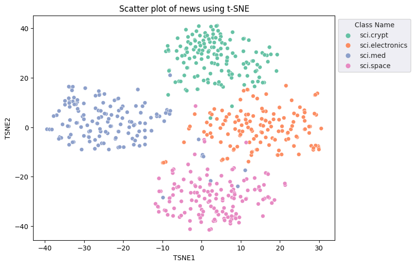
t-분산 확률적 이웃 임베딩 (t-SNE) 접근 방식을 적용하여 차원 축소를 수행합니다. 이 기법은 클러스터 (서로 가까운 지점이 서로 가깝게 유지됨)를 보존하면서 차원 수를 줄입니다. 원본 데이터의 경우 모델은 다른 데이터 포인트가 '이웃'인 분포를 구성하려고 합니다. (예: 의미가 비슷함) 그런 다음 목표 함수를 최적화하여 시각화에서 유사한 분포를 유지합니다.

tsne = TSNE(random_state=0, n_iter=1000)
tsne_results = tsne.fit_transform(X)

df_tsne = pd.DataFrame(tsne_results, columns=['TSNE1', 'TSNE2'])
df_tsne['Class Name'] = df_train['Class Name'] # Add labels column from df_train to df_tsne
df_tsne

fig, ax = plt.subplots(figsize=(8,6)) # Set figsize
sns.set_style('darkgrid', {"grid.color": ".6", "grid.linestyle": ":"})
sns.scatterplot(data=df_tsne, x='TSNE1', y='TSNE2', hue='Class Name', palette='Set2')
sns.move_legend(ax, "upper left", bbox_to_anchor=(1, 1))
plt.title('Scatter plot of news using t-SNE')
plt.xlabel('TSNE1')
plt.ylabel('TSNE2');

png

이상점 감지

어느 포인트가 이상치인지 판단하려면 어떤 포인트가 이상점인지 확인해야 합니다. 먼저 중심, 즉 클러스터의 중심을 나타내는 위치를 찾은 다음 거리를 사용하여 이상점 포인트를 결정합니다.

먼저 각 카테고리의 중심을 구합니다.

def get_centroids(df_tsne):
  # Get the centroid of each cluster
  centroids = df_tsne.groupby('Class Name').mean()
  return centroids

centroids = get_centroids(df_tsne)
centroids

def get_embedding_centroids(df):
  emb_centroids = dict()
  grouped = df.groupby('Class Name')
  for c in grouped.groups:
    sub_df = grouped.get_group(c)
    # Get the centroid value of dimension 768
    emb_centroids[c] = np.mean(sub_df['Embeddings'], axis=0)

  return emb_centroids

emb_c = get_embedding_centroids(df_train)

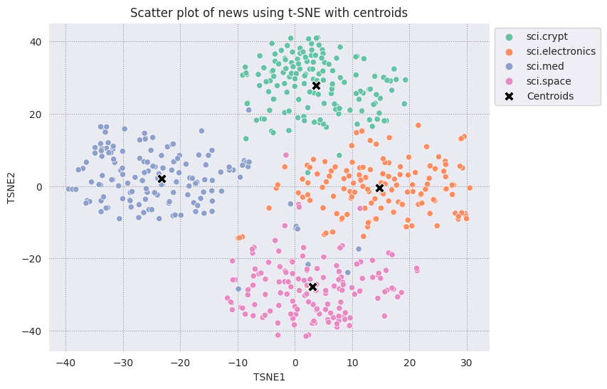
발견한 각 중심을 나머지 점들과 비교해 표시합니다.

# Plot the centroids against the cluster
fig, ax = plt.subplots(figsize=(8,6)) # Set figsize
sns.set_style('darkgrid', {"grid.color": ".6", "grid.linestyle": ":"})
sns.scatterplot(data=df_tsne, x='TSNE1', y='TSNE2', hue='Class Name', palette='Set2');
sns.scatterplot(data=centroids, x='TSNE1', y='TSNE2', color="black", marker='X', s=100, label='Centroids')
sns.move_legend(ax, "upper left", bbox_to_anchor=(1, 1))
plt.title('Scatter plot of news using t-SNE with centroids')
plt.xlabel('TSNE1')
plt.ylabel('TSNE2');

png

반경을 선택합니다. 이 범주의 중심을 벗어나는 값은 이상점으로 간주됩니다.

def calculate_euclidean_distance(p1, p2):
  return np.sqrt(np.sum(np.square(p1 - p2)))

def detect_outlier(df, emb_centroids, radius):
  for idx, row in df.iterrows():
    class_name = row['Class Name'] # Get class name of row
    # Compare centroid distances
    dist = calculate_euclidean_distance(row['Embeddings'],
                                        emb_centroids[class_name])
    df.at[idx, 'Outlier'] = dist > radius

  return len(df[df['Outlier'] == True])

range_ = np.arange(0.3, 0.75, 0.02).round(decimals=2).tolist()
num_outliers = []
for i in range_:
  num_outliers.append(detect_outlier(df_train, emb_c, i))

# Plot range_ and num_outliers
fig = plt.figure(figsize = (14, 8))
plt.rcParams.update({'font.size': 12})
plt.bar(list(map(str, range_)), num_outliers)
plt.title("Number of outliers vs. distance of points from centroid")
plt.xlabel("Distance")
plt.ylabel("Number of outliers")
for i in range(len(range_)):
  plt.text(i, num_outliers[i], num_outliers[i], ha = 'center')

plt.show()

png

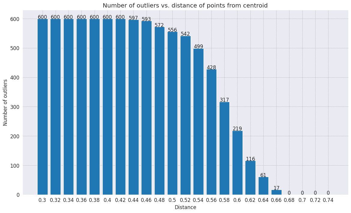
이상 감지기의 민감도에 따라 사용할 반경을 선택할 수 있습니다. 지금은 0.62가 사용되지만 이 값을 변경할 수 있습니다.

# View the points that are outliers
RADIUS = 0.62
detect_outlier(df_train, emb_c, RADIUS)
df_outliers = df_train[df_train['Outlier'] == True]
df_outliers.head()

# Use the index to map the outlier points back to the projected TSNE points
outliers_projected = df_tsne.loc[df_outliers['Outlier'].index]

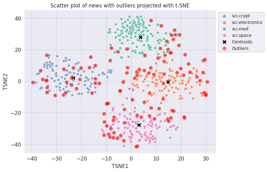
이상점을 표시하고 투명한 빨간색으로 표시합니다.

fig, ax = plt.subplots(figsize=(8,6)) # Set figsize
plt.rcParams.update({'font.size': 10})
sns.set_style('darkgrid', {"grid.color": ".6", "grid.linestyle": ":"})
sns.scatterplot(data=df_tsne, x='TSNE1', y='TSNE2', hue='Class Name', palette='Set2');
sns.scatterplot(data=centroids, x='TSNE1', y='TSNE2', color="black", marker='X', s=100, label='Centroids')
# Draw a red circle around the outliers
sns.scatterplot(data=outliers_projected, x='TSNE1', y='TSNE2', color='red', marker='o', alpha=0.5, s=90, label='Outliers')
sns.move_legend(ax, "upper left", bbox_to_anchor=(1, 1))
plt.title('Scatter plot of news with outliers projected with t-SNE')
plt.xlabel('TSNE1')
plt.ylabel('TSNE2');

png

datafames의 색인 값을 사용하여 각 카테고리에서 이상점이 어떤 모습인지 보여주는 몇 가지 예를 출력합니다. 여기서 각 카테고리의 첫 번째 데이터 포인트가 출력됩니다. 각 카테고리의 다른 포인트를 탐색하여 이상치 또는 이상치로 간주되는 데이터를 확인합니다.

sci_crypt_outliers = df_outliers[df_outliers['Class Name'] == 'sci.crypt']
print(sci_crypt_outliers['Text'].iloc[0])

Re: Source of random bits on a Unix workstation
Lines: 44
Nntp-Posting-Host: sandstorm

>>For your application, what you can do is to encrypt the real-time clock
>>value with a secret key.

Well, almost.... If I only had to solve the problem for myself, and were
willing to have to type in a second password  whenever I
logged in, it could work. However, I'm trying to create a solution that
anyone can use, and which, once installed, is just as effortless to start up
as the non-solution of just using xhost to control access. I've got
religeous problems with storing secret keys on multiuser computers.

>For a good discussion of cryptographically "good" random number
>generators, check out the draft-ietf-security-randomness-00.txt
>Internet Draft, available at your local friendly internet drafts
>repository.

Thanks for the pointer! It was good reading, and I liked the idea of using
several unrelated sources with a strong mixing function. However, unless I
missed something, the only source they suggested 
that seems available, and unguessable by an intruder, when a Unix is
fresh-booted, is I/O buffers related to network traffic. I believe my
solution basically uses that strategy, without requiring me to reach into
the kernel.

>A reasonably source of randomness is the output of a cryptographic
>hash function , when fed with a large amount of
>more-or-less random data. For example, running MD5 on /dev/mem is a
>slow, but random enough, source of random bits; there are bound to be
>128 bits of entropy in the tens  of megabytes of data in
>a modern workstation's memory, as a fair amount of them are system
>timers, i/o buffers, etc.

I heard about this solution, and it sounded good. Then I heard that folks
were experiencing times of 30-60 seconds to run this, on
reasonably-configured workstations. I'm not willing to add that much delay
to someone's login process. My approach  takes
a second or two to run. I'm considering writing the be-all and end-all of
solutions, that launches the MD5, and simultaneously tries to suck bits off
the net, and if the net should be sitting __SO__ idle that it can't get 10K
after compression before MD5 finishes, use the MD5. This way I could have
guaranteed good bits, and a deterministic upper bound on login time, and
still have the common case of login take only a couple of extra seconds.

-Bennett

sci_elec_outliers = df_outliers[df_outliers['Class Name'] == 'sci.electronics']
print(sci_elec_outliers['Text'].iloc[0])

Re: Laser vs Bubblejet?
Reply-To: 
Distribution: world
X-Mailer: cppnews \\(Revision: 1.20 \\)
Organization: null
Lines: 53

Here is a different viewpoint.

> FYI:  The actual horizontal dot placement resoution of an HP
> deskjet is 1/600th inch.  The electronics and dynamics of the ink
> cartridge, however, limit you to generating dots at 300 per inch.
> On almost any paper, the ink wicks more than 1/300th inch anyway.
> 
> The method of depositing and fusing toner of a laster printer
> results in much less spread than ink drop technology.

In practice there is little difference in quality but more care is needed 
with inkjet because smudges etc. can happen.

> It doesn't take much investigation to see that the mechanical and
> electronic complement of a laser printer is more complex than
> inexpensive ink jet printers.  Recall also that laser printers
> offer a much higher throughput:  10 ppm for a laser versus about 1
> ppm for an ink jet printer.

A cheap laser printer does not manage that sort of throughput and on top of 
that how long does the _first_ sheet take to print? Inkjets are faster than 
you say and in both cases the computer often has trouble keeping up with the 
printer. 

A sage said to me: "Do you want one copy or lots of copies?", "One", 
"Inkjet".
 
> Something else to think about is the cost of consumables over the
> life of the printer.  A 3000 page yield toner cartridge is about
> $US 75-80 at discount while HP high capacity 
> cartridges are about $US 22 at discount.  It could be that over the
> life cycle of the printer that consumables for laser printers are
> less than ink jet printers.  It is getting progressively closer
> between the two technologies.  Laser printers are usually desinged
> for higher duty cycles in pages per month and longer product
> replacement cycles.

Paper cost is the same and both can use refills. Long term the laserprinter 
will need some expensive replacement parts  and on top of that 
are the amortisation costs which favour the lowest purchase cost printer.

HP inkjets understand PCL so in many cases a laserjet driver will work if the 
software package has no inkjet driver. 

There is one wild difference between the two printers: a laserprinter is a 
page printer whilst an inkjet is a line printer. This means that a 
laserprinter can rotate graphic images whilst an inkjet cannot. Few drivers 
actually use this facility.


  TC. 
    E-mail:  or

sci_med_outliers = df_outliers[df_outliers['Class Name'] == 'sci.med']
print(sci_med_outliers['Text'].iloc[0])

Re: THE BACK MACHINE - Update
Organization: University of Nebraska--Lincoln 
Lines: 15
Distribution: na
NNTP-Posting-Host: unlinfo.unl.edu

   I have a BACK MACHINE and have had one since January.  While I have not 
found it to be a panacea for my back pain, I think it has helped somewhat. 
It MAINLY acts to stretch muscles in the back and prevent spasms associated
with pain.  I am taking less pain medication than I was previously.  
   The folks at BACK TECHNOLOGIES are VERY reluctant to honor their return 
policy.  They extended my "warranty" period rather than allow me to return 
the machine when, after the first month or so, I was not thrilled with it. 
They encouraged me to continue to use it, abeit less vigourously. 
   Like I said, I can't say it is a cure-all, but it keeps me stretched out
and I am in less pain.
--
***********************************************************************
Dale M. Webb, DVM, PhD           *  97% of the body is water.  The
Veterinary Diagnostic Center     *  other 3% keeps you from drowning.
University of Nebraska, Lincoln  *

sci_space_outliers = df_outliers[df_outliers['Class Name'] == 'sci.space']
print(sci_space_outliers['Text'].iloc[0])

MACH 25 landing site bases?
Article-I.D.: aurora.1993Apr5.193829.1
Organization: University of Alaska Fairbanks
Lines: 7
Nntp-Posting-Host: acad3.alaska.edu

The supersonic booms hear a few months ago over I belive San Fran, heading east
of what I heard, some new super speed Mach 25 aircraft?? What military based
int he direction of flight are there that could handle a Mach 25aircraft on its
landing decent?? Odd question??

==
Michael Adams,  -- I'm not high, just jacked

다음 단계

이제 임베딩을 사용하여 이상 감지기를 만들었습니다. 자체 텍스트 데이터를 사용하여 임베딩으로 시각화하고 이상점을 감지할 수 있는 범위를 선택해 보세요. 시각화 단계를 완료하기 위해 차원을 줄일 수 있습니다. t-SNE는 입력을 클러스터링하는 데 적합하지만 수렴하는 데 더 오래 걸리거나 국소 최솟값에서 멈출 수 있습니다. 이 문제가 발생하면 주성분 분석 (PCA) 기법을 사용할 수도 있습니다.

임베딩을 사용하는 방법을 자세히 알아보려면 다음 튜토리얼을 참조하세요.