การตรวจจับความผิดปกติด้วยการฝัง

ดูใน ai.google.dev

ลองใช้ Colab Notebook

ดูสมุดบันทึกใน GitHub

ภาพรวม

บทแนะนำนี้สาธิตวิธีใช้การฝังจาก Gemini API เพื่อตรวจหาความผิดปกติที่อาจเกิดขึ้นในชุดข้อมูลของคุณ คุณจะเห็นภาพชุดย่อยของชุดข้อมูล 20 Newsgroup โดยใช้ t-SNE และตรวจหาค่าผิดปกตินอกรัศมีที่เฉพาะเจาะจงของจุดศูนย์กลางของคลัสเตอร์แต่ละรายการ

ดูข้อมูลเพิ่มเติมเกี่ยวกับการเริ่มต้นใช้งานการฝังที่สร้างจาก Gemini API ได้ที่การเริ่มต้น Python อย่างรวดเร็ว

ข้อกำหนดเบื้องต้น

โดยคุณสามารถเรียกใช้การเริ่มต้นอย่างรวดเร็วนี้ใน Google Colab ได้

เพื่อให้การเริ่มต้นอย่างรวดเร็วนี้เสร็จสมบูรณ์ในสภาพแวดล้อมการพัฒนาของคุณเอง โปรดตรวจสอบว่าสภาพแวดล้อมของคุณเป็นไปตามข้อกำหนดต่อไปนี้

• Python 3.9 ขึ้นไป
• การติดตั้ง jupyter เพื่อเรียกใช้สมุดบันทึก

ตั้งค่า

ก่อนอื่นให้ดาวน์โหลดและติดตั้งไลบรารี Gemini API Python

pip install -U -q google.generativeai

import re
import tqdm
import numpy as np
import pandas as pd
import matplotlib.pyplot as plt
import seaborn as sns

import google.generativeai as genai

# Used to securely store your API key
from google.colab import userdata

from sklearn.datasets import fetch_20newsgroups
from sklearn.manifold import TSNE

รับคีย์ API

คุณต้องได้รับคีย์ API ก่อนจึงจะใช้ Gemini API ได้ หากยังไม่มี ให้สร้างคีย์ในคลิกเดียวใน Google AI Studio

รับคีย์ API

ใน Colab ให้เพิ่มคีย์ลงในเครื่องมือจัดการความลับใต้ "🔑" ในแผงด้านซ้าย ตั้งชื่อว่า API_KEY

เมื่อมีคีย์ API แล้ว ให้ส่งคีย์ดังกล่าวไปยัง SDK โดยสามารถทำได้สองวิธี:

• ใส่คีย์ในตัวแปรสภาพแวดล้อม GOOGLE_API_KEY (SDK จะดึงคีย์นั้นขึ้นมาโดยอัตโนมัติ)
• ส่งคีย์ไปยัง genai.configure(api_key=...)

genai.configure(api_key=GOOGLE_API_KEY)

for m in genai.list_models():
  if 'embedContent' in m.supported_generation_methods:
    print(m.name)

models/embedding-001
models/embedding-001

เตรียมชุดข้อมูล

ชุดข้อมูลข้อความ 20 กลุ่มข่าวประกอบด้วยโพสต์ของกลุ่มข่าว 18,000 โพสต์ใน 20 หัวข้อที่แบ่งออกเป็นชุดการฝึกและการทดสอบ การแยกระหว่างชุดข้อมูลการฝึกและการทดสอบจะอิงตามข้อความที่โพสต์ก่อนและหลังวันที่ที่ระบุ บทแนะนำนี้ใช้ชุดย่อยการฝึก

newsgroups_train = fetch_20newsgroups(subset='train')

# View list of class names for dataset
newsgroups_train.target_names

['alt.atheism',
 'comp.graphics',
 'comp.os.ms-windows.misc',
 'comp.sys.ibm.pc.hardware',
 'comp.sys.mac.hardware',
 'comp.windows.x',
 'misc.forsale',
 'rec.autos',
 'rec.motorcycles',
 'rec.sport.baseball',
 'rec.sport.hockey',
 'sci.crypt',
 'sci.electronics',
 'sci.med',
 'sci.space',
 'soc.religion.christian',
 'talk.politics.guns',
 'talk.politics.mideast',
 'talk.politics.misc',
 'talk.religion.misc']

นี่เป็นตัวอย่างแรกในชุดการฝึก

idx = newsgroups_train.data[0].index('Lines')
print(newsgroups_train.data[0][idx:])

Lines: 15

 I was wondering if anyone out there could enlighten me on this car I saw
the other day. It was a 2-door sports car, looked to be from the late 60s/
early 70s. It was called a Bricklin. The doors were really small. In addition,
the front bumper was separate from the rest of the body. This is 
all I know. If anyone can tellme a model name, engine specs, years
of production, where this car is made, history, or whatever info you
have on this funky looking car, please e-mail.

Thanks,

- IL
   ---- brought to you by your neighborhood Lerxst ----

# Apply functions to remove names, emails, and extraneous words from data points in newsgroups.data
newsgroups_train.data = [re.sub(r'[\w\.-]+@[\w\.-]+', '', d) for d in newsgroups_train.data] # Remove email
newsgroups_train.data = [re.sub(r"\([^()]*\)", "", d) for d in newsgroups_train.data] # Remove names
newsgroups_train.data = [d.replace("From: ", "") for d in newsgroups_train.data] # Remove "From: "
newsgroups_train.data = [d.replace("\nSubject: ", "") for d in newsgroups_train.data] # Remove "\nSubject: "

# Cut off each text entry after 5,000 characters
newsgroups_train.data = [d[0:5000] if len(d) > 5000 else d for d in newsgroups_train.data]

# Put training points into a dataframe
df_train = pd.DataFrame(newsgroups_train.data, columns=['Text'])
df_train['Label'] = newsgroups_train.target
# Match label to target name index
df_train['Class Name'] = df_train['Label'].map(newsgroups_train.target_names.__getitem__)

df_train

ถัดไป สุ่มตัวอย่างข้อมูลบางส่วนโดยนำจุดข้อมูล 150 จุดในชุดข้อมูลการฝึก และเลือก 2-3 หมวดหมู่ บทแนะนำนี้ใช้หมวดหมู่วิทยาศาสตร์

# Take a sample of each label category from df_train
SAMPLE_SIZE = 150
df_train = (df_train.groupby('Label', as_index = False)
                    .apply(lambda x: x.sample(SAMPLE_SIZE))
                    .reset_index(drop=True))

# Choose categories about science
df_train = df_train[df_train['Class Name'].str.contains('sci')]

# Reset the index
df_train = df_train.reset_index()
df_train

df_train['Class Name'].value_counts()

sci.crypt          150
sci.electronics    150
sci.med            150
sci.space          150
Name: Class Name, dtype: int64

สร้างการฝัง

ในส่วนนี้ คุณจะเห็นวิธีสร้างการฝังสำหรับข้อความต่างๆ ในเฟรมข้อมูลโดยใช้การฝังจาก Gemini API

การเปลี่ยนแปลง API เกี่ยวกับการฝังที่มีการฝังโมเดล-001

สำหรับโมเดลการฝังใหม่ Embed-001 จะมีพารามิเตอร์ประเภทงานใหม่และชื่อที่ไม่บังคับ (ใช้ได้กับ Tasks_type=RETRIEVAL_DOCUMENT เท่านั้น)

พารามิเตอร์ใหม่เหล่านี้จะใช้กับโมเดลการฝังใหม่ล่าสุดเท่านั้น ประเภทงานมีดังนี้

ประเภทงาน	คำอธิบาย
RETRIEVAL_QUERY	ระบุว่าข้อความที่ระบุเป็นคำค้นหาในการตั้งค่าการค้นหา/ดึงข้อมูล
RETRIEVAL_DOCUMENT	ระบุว่าข้อความที่ระบุเป็นเอกสารในการตั้งค่าการค้นหา/ดึงข้อมูล
SEMANTIC_SIMILARITY	ระบุว่าจะใช้ข้อความที่กำหนดสำหรับความคล้ายคลึงกันของข้อความความหมาย (STS)
การจัดประเภท	ระบุว่าจะมีการใช้การฝังสำหรับการจัดประเภท
การคลัสเตอร์	ระบุว่าจะมีการใช้การฝังสำหรับการจัดคลัสเตอร์

from tqdm.auto import tqdm
tqdm.pandas()

from google.api_core import retry

def make_embed_text_fn(model):

  @retry.Retry(timeout=300.0)
  def embed_fn(text: str) -> list[float]:
    # Set the task_type to CLUSTERING.
    embedding = genai.embed_content(model=model,
                                    content=text,
                                    task_type="clustering")['embedding']
    return np.array(embedding)

  return embed_fn

def create_embeddings(df):
  model = 'models/embedding-001'
  df['Embeddings'] = df['Text'].progress_apply(make_embed_text_fn(model))
  return df

df_train = create_embeddings(df_train)
df_train.drop('index', axis=1, inplace=True)

0%|          | 0/600 [00:00<?, ?it/s]

การลดมิติข้อมูล

ขนาดของเวกเตอร์ที่ฝังเอกสารคือ 768 เพื่อให้เห็นภาพวิธีจัดกลุ่มเอกสารที่ฝังไว้ด้วยกัน คุณจะต้องใช้การลดมิติข้อมูลเนื่องจากคุณสามารถแสดงภาพการฝังในพื้นที่ 2 มิติหรือ 3 มิติเท่านั้น เอกสารที่มีบริบทคล้ายกันควรอยู่ใกล้กันในอวกาศ ไม่ใช่เอกสารที่ไม่เหมือนกัน

len(df_train['Embeddings'][0])

768

# Convert df_train['Embeddings'] Pandas series to a np.array of float32
X = np.array(df_train['Embeddings'].to_list(), dtype=np.float32)
X.shape

(600, 768)

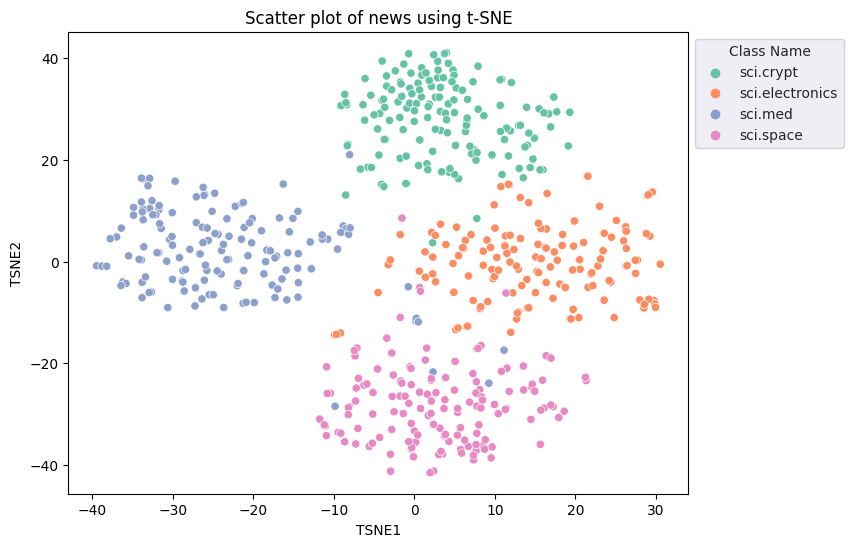
คุณจะใช้วิธี t-Distributed Stochastic Neighbor Embedding (t-SNE) เพื่อดำเนินการลดมิติข้อมูล เทคนิคนี้จะลดจำนวนมิติข้อมูลขณะที่คงคลัสเตอร์ไว้ (จุดที่อยู่ใกล้กันจะอยู่ใกล้กัน) สำหรับข้อมูลต้นฉบับ โมเดลจะพยายามสร้างการกระจายเมื่อเทียบกับจุดข้อมูลอื่นๆ ที่เป็น "เพื่อนบ้าน" (เช่น มีความหมายคล้ายกัน) จากนั้นจะเพิ่มประสิทธิภาพฟังก์ชันที่เป็นวัตถุประสงค์เพื่อรักษาการกระจายที่คล้ายกันในการแสดงภาพ

tsne = TSNE(random_state=0, n_iter=1000)
tsne_results = tsne.fit_transform(X)

df_tsne = pd.DataFrame(tsne_results, columns=['TSNE1', 'TSNE2'])
df_tsne['Class Name'] = df_train['Class Name'] # Add labels column from df_train to df_tsne
df_tsne

fig, ax = plt.subplots(figsize=(8,6)) # Set figsize
sns.set_style('darkgrid', {"grid.color": ".6", "grid.linestyle": ":"})
sns.scatterplot(data=df_tsne, x='TSNE1', y='TSNE2', hue='Class Name', palette='Set2')
sns.move_legend(ax, "upper left", bbox_to_anchor=(1, 1))
plt.title('Scatter plot of news using t-SNE')
plt.xlabel('TSNE1')
plt.ylabel('TSNE2');

การตรวจจับ Outlier

ในการพิจารณาว่าจุดใดที่มีความผิดปกติ คุณจะเป็นผู้ตัดสินว่าจุดใดเป็นค่าอินไลน์และค่าผิดปกติ เริ่มด้วยการหาจุดศูนย์กลางหรือตำแหน่งที่แทนจุดศูนย์กลางของคลัสเตอร์ และใช้ระยะทางเพื่อกำหนดจุดที่มีค่าผิดปกติ

เริ่มต้นด้วยการหาจุดศูนย์กลางของแต่ละหมวดหมู่

def get_centroids(df_tsne):
  # Get the centroid of each cluster
  centroids = df_tsne.groupby('Class Name').mean()
  return centroids

centroids = get_centroids(df_tsne)
centroids

def get_embedding_centroids(df):
  emb_centroids = dict()
  grouped = df.groupby('Class Name')
  for c in grouped.groups:
    sub_df = grouped.get_group(c)
    # Get the centroid value of dimension 768
    emb_centroids[c] = np.mean(sub_df['Embeddings'], axis=0)

  return emb_centroids

emb_c = get_embedding_centroids(df_train)

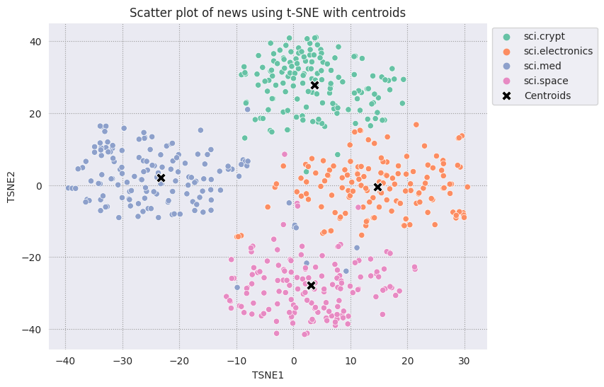
วาดเส้นศูนย์กลางแต่ละจุดที่พบเทียบกับจุดที่เหลือ

# Plot the centroids against the cluster
fig, ax = plt.subplots(figsize=(8,6)) # Set figsize
sns.set_style('darkgrid', {"grid.color": ".6", "grid.linestyle": ":"})
sns.scatterplot(data=df_tsne, x='TSNE1', y='TSNE2', hue='Class Name', palette='Set2');
sns.scatterplot(data=centroids, x='TSNE1', y='TSNE2', color="black", marker='X', s=100, label='Centroids')
sns.move_legend(ax, "upper left", bbox_to_anchor=(1, 1))
plt.title('Scatter plot of news using t-SNE with centroids')
plt.xlabel('TSNE1')
plt.ylabel('TSNE2');

เลือกรัศมี สิ่งใดก็ตามที่อยู่นอกเหนือขอบเขตนี้จากจุดศูนย์กลางของหมวดหมู่นั้นจะถือว่าเป็นค่าผิดปกติ

def calculate_euclidean_distance(p1, p2):
  return np.sqrt(np.sum(np.square(p1 - p2)))

def detect_outlier(df, emb_centroids, radius):
  for idx, row in df.iterrows():
    class_name = row['Class Name'] # Get class name of row
    # Compare centroid distances
    dist = calculate_euclidean_distance(row['Embeddings'],
                                        emb_centroids[class_name])
    df.at[idx, 'Outlier'] = dist > radius

  return len(df[df['Outlier'] == True])

range_ = np.arange(0.3, 0.75, 0.02).round(decimals=2).tolist()
num_outliers = []
for i in range_:
  num_outliers.append(detect_outlier(df_train, emb_c, i))

# Plot range_ and num_outliers
fig = plt.figure(figsize = (14, 8))
plt.rcParams.update({'font.size': 12})
plt.bar(list(map(str, range_)), num_outliers)
plt.title("Number of outliers vs. distance of points from centroid")
plt.xlabel("Distance")
plt.ylabel("Number of outliers")
for i in range(len(range_)):
  plt.text(i, num_outliers[i], num_outliers[i], ha = 'center')

plt.show()

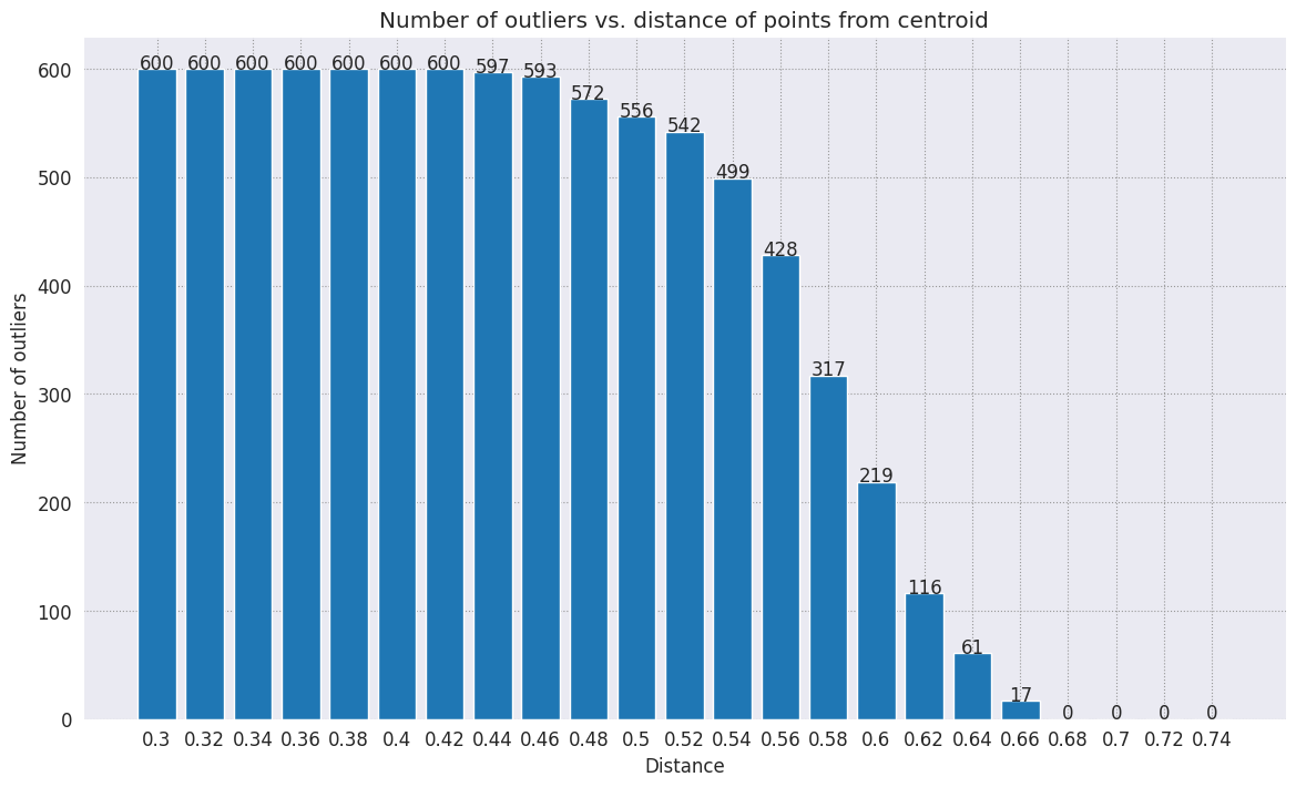
คุณเลือกรัศมีที่ต้องการใช้ได้ โดยขึ้นอยู่กับความไวที่คุณต้องการให้ตัวตรวจจับความผิดปกติ ตอนนี้ใช้ 0.62 ไปแล้ว แต่คุณเปลี่ยนค่านี้ได้

# View the points that are outliers
RADIUS = 0.62
detect_outlier(df_train, emb_c, RADIUS)
df_outliers = df_train[df_train['Outlier'] == True]
df_outliers.head()

# Use the index to map the outlier points back to the projected TSNE points
outliers_projected = df_tsne.loc[df_outliers['Outlier'].index]

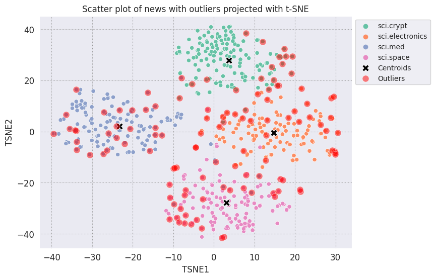
พล็อตค่าผิดปกติและแสดงถึงค่าเหล่านั้นโดยใช้สีแดงโปร่งแสง

fig, ax = plt.subplots(figsize=(8,6)) # Set figsize
plt.rcParams.update({'font.size': 10})
sns.set_style('darkgrid', {"grid.color": ".6", "grid.linestyle": ":"})
sns.scatterplot(data=df_tsne, x='TSNE1', y='TSNE2', hue='Class Name', palette='Set2');
sns.scatterplot(data=centroids, x='TSNE1', y='TSNE2', color="black", marker='X', s=100, label='Centroids')
# Draw a red circle around the outliers
sns.scatterplot(data=outliers_projected, x='TSNE1', y='TSNE2', color='red', marker='o', alpha=0.5, s=90, label='Outliers')
sns.move_legend(ax, "upper left", bbox_to_anchor=(1, 1))
plt.title('Scatter plot of news with outliers projected with t-SNE')
plt.xlabel('TSNE1')
plt.ylabel('TSNE2');

ใช้ค่าดัชนีของ Datafame เพื่อพิมพ์ตัวอย่างลักษณะที่ค่าผิดปกติในแต่ละหมวดหมู่ โดยจะมีการพิมพ์จุดข้อมูลแรกจากแต่ละหมวดหมู่ออกมา สำรวจจุดอื่นๆ ในแต่ละหมวดหมู่เพื่อดูข้อมูลที่ถือว่าเป็นค่าผิดปกติหรือความผิดปกติ

sci_crypt_outliers = df_outliers[df_outliers['Class Name'] == 'sci.crypt']
print(sci_crypt_outliers['Text'].iloc[0])

Re: Source of random bits on a Unix workstation
Lines: 44
Nntp-Posting-Host: sandstorm

>>For your application, what you can do is to encrypt the real-time clock
>>value with a secret key.

Well, almost.... If I only had to solve the problem for myself, and were
willing to have to type in a second password  whenever I
logged in, it could work. However, I'm trying to create a solution that
anyone can use, and which, once installed, is just as effortless to start up
as the non-solution of just using xhost to control access. I've got
religeous problems with storing secret keys on multiuser computers.

>For a good discussion of cryptographically "good" random number
>generators, check out the draft-ietf-security-randomness-00.txt
>Internet Draft, available at your local friendly internet drafts
>repository.

Thanks for the pointer! It was good reading, and I liked the idea of using
several unrelated sources with a strong mixing function. However, unless I
missed something, the only source they suggested 
that seems available, and unguessable by an intruder, when a Unix is
fresh-booted, is I/O buffers related to network traffic. I believe my
solution basically uses that strategy, without requiring me to reach into
the kernel.

>A reasonably source of randomness is the output of a cryptographic
>hash function , when fed with a large amount of
>more-or-less random data. For example, running MD5 on /dev/mem is a
>slow, but random enough, source of random bits; there are bound to be
>128 bits of entropy in the tens  of megabytes of data in
>a modern workstation's memory, as a fair amount of them are system
>timers, i/o buffers, etc.

I heard about this solution, and it sounded good. Then I heard that folks
were experiencing times of 30-60 seconds to run this, on
reasonably-configured workstations. I'm not willing to add that much delay
to someone's login process. My approach  takes
a second or two to run. I'm considering writing the be-all and end-all of
solutions, that launches the MD5, and simultaneously tries to suck bits off
the net, and if the net should be sitting __SO__ idle that it can't get 10K
after compression before MD5 finishes, use the MD5. This way I could have
guaranteed good bits, and a deterministic upper bound on login time, and
still have the common case of login take only a couple of extra seconds.

-Bennett

sci_elec_outliers = df_outliers[df_outliers['Class Name'] == 'sci.electronics']
print(sci_elec_outliers['Text'].iloc[0])

Re: Laser vs Bubblejet?
Reply-To: 
Distribution: world
X-Mailer: cppnews \\(Revision: 1.20 \\)
Organization: null
Lines: 53

Here is a different viewpoint.

> FYI:  The actual horizontal dot placement resoution of an HP
> deskjet is 1/600th inch.  The electronics and dynamics of the ink
> cartridge, however, limit you to generating dots at 300 per inch.
> On almost any paper, the ink wicks more than 1/300th inch anyway.
> 
> The method of depositing and fusing toner of a laster printer
> results in much less spread than ink drop technology.

In practice there is little difference in quality but more care is needed 
with inkjet because smudges etc. can happen.

> It doesn't take much investigation to see that the mechanical and
> electronic complement of a laser printer is more complex than
> inexpensive ink jet printers.  Recall also that laser printers
> offer a much higher throughput:  10 ppm for a laser versus about 1
> ppm for an ink jet printer.

A cheap laser printer does not manage that sort of throughput and on top of 
that how long does the _first_ sheet take to print? Inkjets are faster than 
you say and in both cases the computer often has trouble keeping up with the 
printer. 

A sage said to me: "Do you want one copy or lots of copies?", "One", 
"Inkjet".
 
> Something else to think about is the cost of consumables over the
> life of the printer.  A 3000 page yield toner cartridge is about
> $US 75-80 at discount while HP high capacity 
> cartridges are about $US 22 at discount.  It could be that over the
> life cycle of the printer that consumables for laser printers are
> less than ink jet printers.  It is getting progressively closer
> between the two technologies.  Laser printers are usually desinged
> for higher duty cycles in pages per month and longer product
> replacement cycles.

Paper cost is the same and both can use refills. Long term the laserprinter 
will need some expensive replacement parts  and on top of that 
are the amortisation costs which favour the lowest purchase cost printer.

HP inkjets understand PCL so in many cases a laserjet driver will work if the 
software package has no inkjet driver. 

There is one wild difference between the two printers: a laserprinter is a 
page printer whilst an inkjet is a line printer. This means that a 
laserprinter can rotate graphic images whilst an inkjet cannot. Few drivers 
actually use this facility.


  TC. 
    E-mail:  or

sci_med_outliers = df_outliers[df_outliers['Class Name'] == 'sci.med']
print(sci_med_outliers['Text'].iloc[0])

Re: THE BACK MACHINE - Update
Organization: University of Nebraska--Lincoln 
Lines: 15
Distribution: na
NNTP-Posting-Host: unlinfo.unl.edu

   I have a BACK MACHINE and have had one since January.  While I have not 
found it to be a panacea for my back pain, I think it has helped somewhat. 
It MAINLY acts to stretch muscles in the back and prevent spasms associated
with pain.  I am taking less pain medication than I was previously.  
   The folks at BACK TECHNOLOGIES are VERY reluctant to honor their return 
policy.  They extended my "warranty" period rather than allow me to return 
the machine when, after the first month or so, I was not thrilled with it. 
They encouraged me to continue to use it, abeit less vigourously. 
   Like I said, I can't say it is a cure-all, but it keeps me stretched out
and I am in less pain.
--
***********************************************************************
Dale M. Webb, DVM, PhD           *  97% of the body is water.  The
Veterinary Diagnostic Center     *  other 3% keeps you from drowning.
University of Nebraska, Lincoln  *

sci_space_outliers = df_outliers[df_outliers['Class Name'] == 'sci.space']
print(sci_space_outliers['Text'].iloc[0])

MACH 25 landing site bases?
Article-I.D.: aurora.1993Apr5.193829.1
Organization: University of Alaska Fairbanks
Lines: 7
Nntp-Posting-Host: acad3.alaska.edu

The supersonic booms hear a few months ago over I belive San Fran, heading east
of what I heard, some new super speed Mach 25 aircraft?? What military based
int he direction of flight are there that could handle a Mach 25aircraft on its
landing decent?? Odd question??

==
Michael Adams,  -- I'm not high, just jacked

ขั้นตอนถัดไป

ตอนนี้คุณได้สร้างตัวตรวจจับความผิดปกติโดยใช้การฝังแล้ว ลองใช้ข้อมูลแบบข้อความของคุณเองเพื่อแสดงภาพข้อมูลเหล่านั้นเป็นการฝัง และเลือกขอบเขตที่คุณสามารถตรวจจับความผิดปกติได้ คุณสามารถลดมิติข้อมูลเพื่อทำตามขั้นตอนการแสดงภาพให้เสร็จสมบูรณ์ โปรดทราบว่า t-SNE เหมาะสำหรับการจัดกลุ่มอินพุต แต่อาจใช้เวลานานขึ้นในการบรรจบกันหรืออาจค้างที่ขนาดเล็กที่สุดในเครื่อง หากพบปัญหานี้ คุณอาจลองใช้อีกเทคนิคหนึ่งคือการวิเคราะห์องค์ประกอบหลัก (PCA)

หากต้องการดูข้อมูลเพิ่มเติมเกี่ยวกับวิธีใช้การฝัง โปรดดูบทแนะนำอื่นๆ เหล่านี้

• การจัดกลุ่มด้วยการฝัง
• การค้นหาเอกสารด้วยการฝัง
• การฝึกตัวแยกประเภทข้อความด้วยการฝัง