
|
|
|
 Notebook auf GitHub ansehen Notebook auf GitHub ansehen
|
Übersicht
In dieser Anleitung wird gezeigt, wie Sie mithilfe der Einbettungen der Gemini API potenzielle Ausreißer in Ihrem Dataset erkennen. Sie visualisieren eine Teilmenge der 20 Newsgroup-Datasets mithilfe von t-SNE und erkennen Ausreißer außerhalb eines bestimmten Radius des zentralen Punkts jedes kategorialen Clusters.
Weitere Informationen zu den ersten Schritten mit Einbettungen, die mit der Gemini API generiert werden, finden Sie in der Python-Kurzanleitung.
Vorbereitung
Sie können diese Kurzanleitung in Google Colab ausführen.
Wenn Sie diese Kurzanleitung in Ihrer eigenen Entwicklungsumgebung ausführen möchten, muss Ihre Umgebung die folgenden Anforderungen erfüllen:
- Python 3.9 oder höher
- Eine Installation von
jupyterzum Ausführen des Notebooks.
Einrichtung
Laden Sie zuerst die Gemini API-Python-Bibliothek herunter und installieren Sie sie.
pip install -U -q google.generativeai
import re
import tqdm
import numpy as np
import pandas as pd
import matplotlib.pyplot as plt
import seaborn as sns

import google.generativeai as genai

# Used to securely store your API key
from google.colab import userdata

from sklearn.datasets import fetch_20newsgroups
from sklearn.manifold import TSNE
API-Schlüssel anfordern
Bevor Sie die Gemini API verwenden können, müssen Sie einen API-Schlüssel abrufen. Wenn Sie noch keinen Schlüssel haben, können Sie mit einem Klick in Google AI Studio einen Schlüssel erstellen.
Fügen Sie den Schlüssel in Colab dem Secret-Manager unter dem Menüpunkt „🚀“ hinzu. im linken Bereich. Geben Sie ihr den Namen API_KEY.
Sobald Sie den API-Schlüssel haben, übergeben Sie ihn an das SDK. Dafür haben Sie die beiden folgenden Möglichkeiten:
- Fügen Sie den Schlüssel in die Umgebungsvariable
GOOGLE_API_KEYein. Das SDK ruft ihn dort automatisch ab. - Übergib den Schlüssel an
genai.configure(api_key=...)
genai.configure(api_key=GOOGLE_API_KEY)
for m in genai.list_models():
  if 'embedContent' in m.supported_generation_methods:
    print(m.name)
models/embedding-001
models/embedding-001
Dataset vorbereiten
Das Text-Dataset für 20 Newsgroups enthält 18.000 Newsgroups zu 20 Themen,die in Trainings- und Test-Datasets aufgeteilt sind. Die Aufteilung zwischen Trainings- und Test-Datasets basiert auf Nachrichten, die vor und nach einem bestimmten Datum veröffentlicht wurden. In dieser Anleitung wird die Trainingsteilmenge verwendet.
newsgroups_train = fetch_20newsgroups(subset='train')

# View list of class names for dataset
newsgroups_train.target_names
['alt.atheism',
 'comp.graphics',
 'comp.os.ms-windows.misc',
 'comp.sys.ibm.pc.hardware',
 'comp.sys.mac.hardware',
 'comp.windows.x',
 'misc.forsale',
 'rec.autos',
 'rec.motorcycles',
 'rec.sport.baseball',
 'rec.sport.hockey',
 'sci.crypt',
 'sci.electronics',
 'sci.med',
 'sci.space',
 'soc.religion.christian',
 'talk.politics.guns',
 'talk.politics.mideast',
 'talk.politics.misc',
 'talk.religion.misc']
Hier ist das erste Beispiel im Trainings-Dataset.
idx = newsgroups_train.data[0].index('Lines')
print(newsgroups_train.data[0][idx:])
Lines: 15

 I was wondering if anyone out there could enlighten me on this car I saw
the other day. It was a 2-door sports car, looked to be from the late 60s/
early 70s. It was called a Bricklin. The doors were really small. In addition,
the front bumper was separate from the rest of the body. This is
all I know. If anyone can tellme a model name, engine specs, years
of production, where this car is made, history, or whatever info you
have on this funky looking car, please e-mail.

Thanks,

- IL
   ---- brought to you by your neighborhood Lerxst ----
# Apply functions to remove names, emails, and extraneous words from data points in newsgroups.data
newsgroups_train.data = [re.sub(r'[\w\.-]+@[\w\.-]+', '', d) for d in newsgroups_train.data] # Remove email
newsgroups_train.data = [re.sub(r"\([^()]*\)", "", d) for d in newsgroups_train.data] # Remove names
newsgroups_train.data = [d.replace("From: ", "") for d in newsgroups_train.data] # Remove "From: "
newsgroups_train.data = [d.replace("\nSubject: ", "") for d in newsgroups_train.data] # Remove "\nSubject: "

# Cut off each text entry after 5,000 characters
newsgroups_train.data = [d[0:5000] if len(d) > 5000 else d for d in newsgroups_train.data]
# Put training points into a dataframe
df_train = pd.DataFrame(newsgroups_train.data, columns=['Text'])
df_train['Label'] = newsgroups_train.target
# Match label to target name index
df_train['Class Name'] = df_train['Label'].map(newsgroups_train.target_names.__getitem__)

df_train
Als Nächstes nehmen Sie einige der Daten stichprobenartig auf, indem Sie 150 Datenpunkte im Trainings-Dataset verwenden und einige Kategorien auswählen. In dieser Anleitung werden die Wissenschaftskategorien verwendet.
# Take a sample of each label category from df_train
SAMPLE_SIZE = 150
df_train = (df_train.groupby('Label', as_index = False)
                    .apply(lambda x: x.sample(SAMPLE_SIZE))
                    .reset_index(drop=True))

# Choose categories about science
df_train = df_train[df_train['Class Name'].str.contains('sci')]

# Reset the index
df_train = df_train.reset_index()
df_train
df_train['Class Name'].value_counts()
sci.crypt          150
sci.electronics    150
sci.med            150
sci.space          150
Name: Class Name, dtype: int64
Einbettungen erstellen
In diesem Abschnitt erfahren Sie, wie Sie mithilfe der Einbettungen aus der Gemini API Einbettungen für die verschiedenen Texte im DataFrame generieren.
API-Änderungen an Einbettungen mit Modell „embedding-001“
Für das neue Einbettungsmodell „embedding-001“ gibt es einen neuen Aufgabentypparameter und den optionalen Titel (nur gültig bei „task_type=RETRIEVAL_DOCUMENT“).
Diese neuen Parameter gelten nur für die neuesten Einbettungsmodelle.Es gibt folgende Aufgabentypen:
| Aufgabentyp | Beschreibung |
|---|---|
| RETRIEVAL_QUERY | Gibt an, dass der angegebene Text eine Abfrage in einer Such-/Abrufeinstellung ist. |
| RETRIEVAL_DOCUMENT | Gibt an, dass der angegebene Text ein Dokument in einer Such-/Abrufeinstellung ist. |
| SEMANTIC_SIMILARITY | Gibt an, dass der angegebene Text für die Bestimmung der semantischen Textähnlichkeit (Semantic Textual Similarity, STS) verwendet wird. |
| KLASSIFIZIERUNG | Gibt an, dass die Einbettungen zur Klassifizierung verwendet werden. |
| Clustering | Gibt an, dass die Einbettungen für das Clustering verwendet werden. |
from tqdm.auto import tqdm
tqdm.pandas()

from google.api_core import retry

def make_embed_text_fn(model):

  @retry.Retry(timeout=300.0)
  def embed_fn(text: str) -> list[float]:
    # Set the task_type to CLUSTERING.
    embedding = genai.embed_content(model=model,
                                    content=text,
                                    task_type="clustering")['embedding']
    return np.array(embedding)

  return embed_fn

def create_embeddings(df):
  model = 'models/embedding-001'
  df['Embeddings'] = df['Text'].progress_apply(make_embed_text_fn(model))
  return df

df_train = create_embeddings(df_train)
df_train.drop('index', axis=1, inplace=True)
0%| | 0/600 [00:00<?, ?it/s]
Dimensionalitätsreduktion
Die Dimension des Dokumenteinbettungsvektors beträgt 768. Um zu visualisieren, wie die eingebetteten Dokumente gruppiert werden, müssen Sie die Dimensionalität reduzieren, da die Einbettungen nur im 2D- oder 3D-Raum visualisiert werden können. Kontextbezogene ähnliche Dokumente sollten räumlich näher beieinander liegen, im Gegensatz zu Dokumenten, die sich nicht so ähnlich sind.
len(df_train['Embeddings'][0])
768
# Convert df_train['Embeddings'] Pandas series to a np.array of float32
X = np.array(df_train['Embeddings'].to_list(), dtype=np.float32)
X.shape
(600, 768)
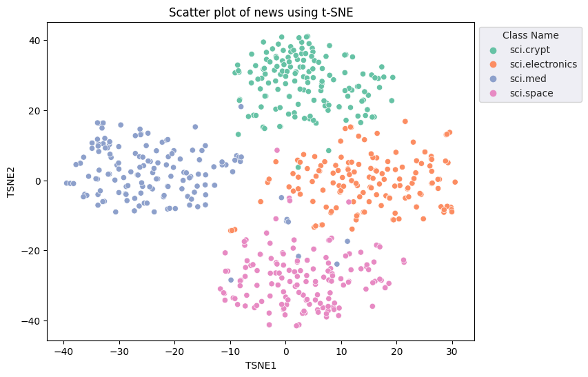
Sie wenden den t-Distributed Stochastic Neighbor Embedding (t-SNE)-Ansatz an, um eine Dimensionalitätsreduzierung durchzuführen. Mit diesem Verfahren wird die Anzahl der Dimensionen reduziert und gleichzeitig Cluster erhalten (d. h. nahe beieinander liegende Punkte bleiben nah beieinander). Für die Originaldaten versucht das Modell, eine Verteilung zu konstruieren, über die andere Datenpunkte „Nachbarn“ sind (haben z.B. eine ähnliche Bedeutung). Dann wird eine Zielfunktion optimiert, um eine ähnliche Verteilung in der Visualisierung beizubehalten.
tsne = TSNE(random_state=0, n_iter=1000)
tsne_results = tsne.fit_transform(X)
df_tsne = pd.DataFrame(tsne_results, columns=['TSNE1', 'TSNE2'])
df_tsne['Class Name'] = df_train['Class Name'] # Add labels column from df_train to df_tsne
df_tsne
fig, ax = plt.subplots(figsize=(8,6)) # Set figsize
sns.set_style('darkgrid', {"grid.color": ".6", "grid.linestyle": ":"})
sns.scatterplot(data=df_tsne, x='TSNE1', y='TSNE2', hue='Class Name', palette='Set2')
sns.move_legend(ax, "upper left", bbox_to_anchor=(1, 1))
plt.title('Scatter plot of news using t-SNE')
plt.xlabel('TSNE1')
plt.ylabel('TSNE2');
Ausreißererkennung
Um festzustellen, welche Punkte anomal sind, ermitteln Sie, welche Punkte Ausreißer und Ausreißer sind. Ermitteln Sie zuerst den Schwerpunkt oder Standort, der den Mittelpunkt des Clusters darstellt, und ermitteln Sie anhand der Entfernung die Punkte, die Ausreißer sind.
Ermitteln Sie zunächst den Schwerpunkt jeder Kategorie.
def get_centroids(df_tsne):
  # Get the centroid of each cluster
  centroids = df_tsne.groupby('Class Name').mean()
  return centroids

centroids = get_centroids(df_tsne)
centroids
def get_embedding_centroids(df):
  emb_centroids = dict()
  grouped = df.groupby('Class Name')
  for c in grouped.groups:
    sub_df = grouped.get_group(c)
    # Get the centroid value of dimension 768
    emb_centroids[c] = np.mean(sub_df['Embeddings'], axis=0)

  return emb_centroids
emb_c = get_embedding_centroids(df_train)
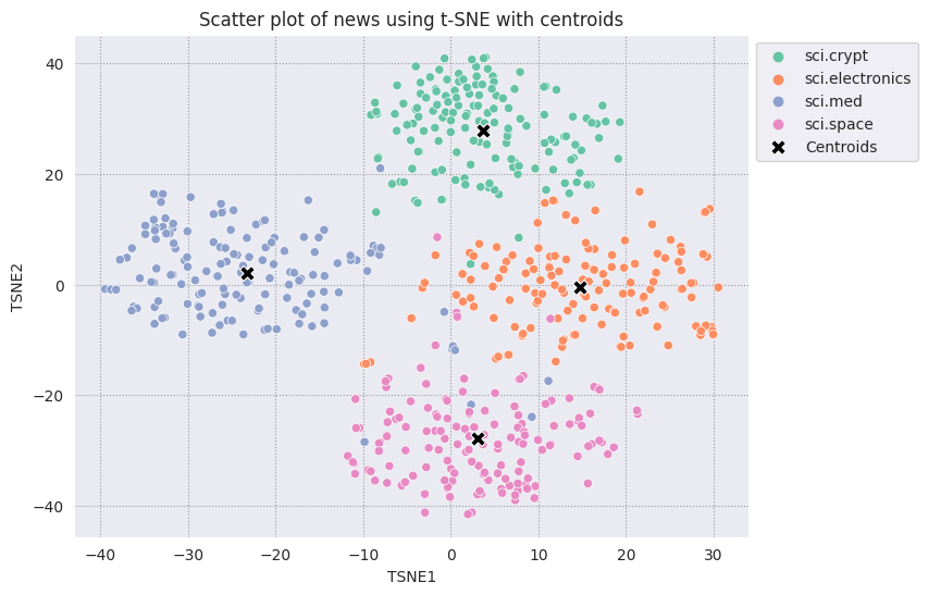
Stellen Sie jeden gefundenen Schwerpunkt mit den anderen Punkten dar.
# Plot the centroids against the cluster
fig, ax = plt.subplots(figsize=(8,6)) # Set figsize
sns.set_style('darkgrid', {"grid.color": ".6", "grid.linestyle": ":"})
sns.scatterplot(data=df_tsne, x='TSNE1', y='TSNE2', hue='Class Name', palette='Set2');
sns.scatterplot(data=centroids, x='TSNE1', y='TSNE2', color="black", marker='X', s=100, label='Centroids')
sns.move_legend(ax, "upper left", bbox_to_anchor=(1, 1))
plt.title('Scatter plot of news using t-SNE with centroids')
plt.xlabel('TSNE1')
plt.ylabel('TSNE2');
Wählen Sie einen Umkreis aus. Alles jenseits dieser Grenze vom Schwerpunkt dieser Kategorie wird als Ausreißer betrachtet.
def calculate_euclidean_distance(p1, p2):
  return np.sqrt(np.sum(np.square(p1 - p2)))

def detect_outlier(df, emb_centroids, radius):
  for idx, row in df.iterrows():
    class_name = row['Class Name'] # Get class name of row
    # Compare centroid distances
    dist = calculate_euclidean_distance(row['Embeddings'],
                                        emb_centroids[class_name])
    df.at[idx, 'Outlier'] = dist > radius

  return len(df[df['Outlier'] == True])
range_ = np.arange(0.3, 0.75, 0.02).round(decimals=2).tolist()
num_outliers = []
for i in range_:
  num_outliers.append(detect_outlier(df_train, emb_c, i))
# Plot range_ and num_outliers
fig = plt.figure(figsize = (14, 8))
plt.rcParams.update({'font.size': 12})
plt.bar(list(map(str, range_)), num_outliers)
plt.title("Number of outliers vs. distance of points from centroid")
plt.xlabel("Distance")
plt.ylabel("Number of outliers")
for i in range(len(range_)):
  plt.text(i, num_outliers[i], num_outliers[i], ha = 'center')

plt.show()
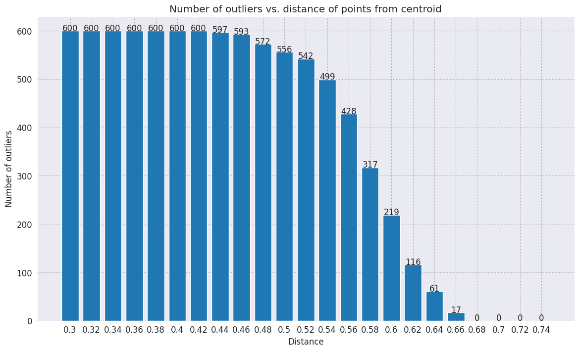
Je nachdem, wie empfindlich der Anomaliedetektor sein soll, können Sie den gewünschten Radius auswählen. Derzeit wird 0, 62 verwendet, Sie können diesen Wert jedoch ändern.
# View the points that are outliers
RADIUS = 0.62
detect_outlier(df_train, emb_c, RADIUS)
df_outliers = df_train[df_train['Outlier'] == True]
df_outliers.head()
# Use the index to map the outlier points back to the projected TSNE points
outliers_projected = df_tsne.loc[df_outliers['Outlier'].index]
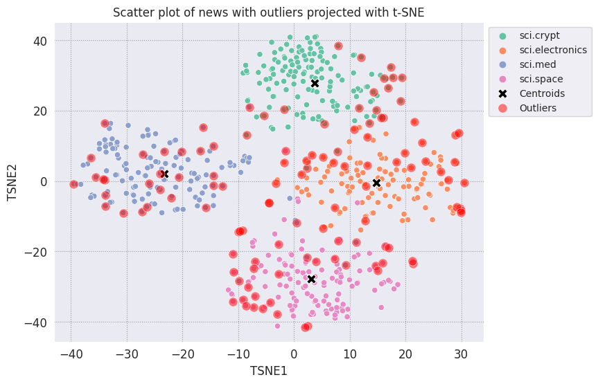
Stellen Sie die Ausreißer dar und kennzeichnen Sie sie mit einer transparenten roten Farbe.
fig, ax = plt.subplots(figsize=(8,6)) # Set figsize
plt.rcParams.update({'font.size': 10})
sns.set_style('darkgrid', {"grid.color": ".6", "grid.linestyle": ":"})
sns.scatterplot(data=df_tsne, x='TSNE1', y='TSNE2', hue='Class Name', palette='Set2');
sns.scatterplot(data=centroids, x='TSNE1', y='TSNE2', color="black", marker='X', s=100, label='Centroids')
# Draw a red circle around the outliers
sns.scatterplot(data=outliers_projected, x='TSNE1', y='TSNE2', color='red', marker='o', alpha=0.5, s=90, label='Outliers')
sns.move_legend(ax, "upper left", bbox_to_anchor=(1, 1))
plt.title('Scatter plot of news with outliers projected with t-SNE')
plt.xlabel('TSNE1')
plt.ylabel('TSNE2');
Verwenden Sie die Indexwerte der Datafames, um einige Beispiele dafür auszudrucken, wie Ausreißer in den einzelnen Kategorien aussehen können. Hier wird der erste Datenpunkt jeder Kategorie ausgedruckt. Untersuchen Sie andere Punkte in jeder Kategorie, um Daten zu sehen, die als Ausreißer oder Anomalien betrachtet werden.
sci_crypt_outliers = df_outliers[df_outliers['Class Name'] == 'sci.crypt']
print(sci_crypt_outliers['Text'].iloc[0])
Re: Source of random bits on a Unix workstation
Lines: 44
Nntp-Posting-Host: sandstorm

>>For your application, what you can do is to encrypt the real-time clock
>>value with a secret key.

Well, almost.... If I only had to solve the problem for myself, and were
willing to have to type in a second password  whenever I
logged in, it could work. However, I'm trying to create a solution that
anyone can use, and which, once installed, is just as effortless to start up
as the non-solution of just using xhost to control access. I've got
religeous problems with storing secret keys on multiuser computers.

>For a good discussion of cryptographically "good" random number
>generators, check out the draft-ietf-security-randomness-00.txt
>Internet Draft, available at your local friendly internet drafts
>repository.

Thanks for the pointer! It was good reading, and I liked the idea of using
several unrelated sources with a strong mixing function. However, unless I
missed something, the only source they suggested
that seems available, and unguessable by an intruder, when a Unix is
fresh-booted, is I/O buffers related to network traffic. I believe my
solution basically uses that strategy, without requiring me to reach into
the kernel.

>A reasonably source of randomness is the output of a cryptographic
>hash function , when fed with a large amount of
>more-or-less random data. For example, running MD5 on /dev/mem is a
>slow, but random enough, source of random bits; there are bound to be
>128 bits of entropy in the tens  of megabytes of data in
>a modern workstation's memory, as a fair amount of them are system
>timers, i/o buffers, etc.

I heard about this solution, and it sounded good. Then I heard that folks
were experiencing times of 30-60 seconds to run this, on
reasonably-configured workstations. I'm not willing to add that much delay
to someone's login process. My approach  takes
a second or two to run. I'm considering writing the be-all and end-all of
solutions, that launches the MD5, and simultaneously tries to suck bits off
the net, and if the net should be sitting __SO__ idle that it can't get 10K
after compression before MD5 finishes, use the MD5. This way I could have
guaranteed good bits, and a deterministic upper bound on login time, and
still have the common case of login take only a couple of extra seconds.

-Bennett
sci_elec_outliers = df_outliers[df_outliers['Class Name'] == 'sci.electronics']
print(sci_elec_outliers['Text'].iloc[0])
Re: Laser vs Bubblejet?
Reply-To:
Distribution: world
X-Mailer: cppnews \\(Revision: 1.20 \\)
Organization: null
Lines: 53

Here is a different viewpoint.

> FYI:  The actual horizontal dot placement resoution of an HP
> deskjet is 1/600th inch.  The electronics and dynamics of the ink
> cartridge, however, limit you to generating dots at 300 per inch.
> On almost any paper, the ink wicks more than 1/300th inch anyway.
>
> The method of depositing and fusing toner of a laster printer
> results in much less spread than ink drop technology.

In practice there is little difference in quality but more care is needed
with inkjet because smudges etc. can happen.

> It doesn't take much investigation to see that the mechanical and
> electronic complement of a laser printer is more complex than
> inexpensive ink jet printers.  Recall also that laser printers
> offer a much higher throughput:  10 ppm for a laser versus about 1
> ppm for an ink jet printer.

A cheap laser printer does not manage that sort of throughput and on top of
that how long does the _first_ sheet take to print? Inkjets are faster than
you say and in both cases the computer often has trouble keeping up with the
printer.

A sage said to me: "Do you want one copy or lots of copies?", "One",
"Inkjet".

> Something else to think about is the cost of consumables over the
> life of the printer.  A 3000 page yield toner cartridge is about
> $US 75-80 at discount while HP high capacity
> cartridges are about $US 22 at discount.  It could be that over the
> life cycle of the printer that consumables for laser printers are
> less than ink jet printers.  It is getting progressively closer
> between the two technologies.  Laser printers are usually desinged
> for higher duty cycles in pages per month and longer product
> replacement cycles.

Paper cost is the same and both can use refills. Long term the laserprinter
will need some expensive replacement parts  and on top of that
are the amortisation costs which favour the lowest purchase cost printer.

HP inkjets understand PCL so in many cases a laserjet driver will work if the
software package has no inkjet driver.

There is one wild difference between the two printers: a laserprinter is a
page printer whilst an inkjet is a line printer. This means that a
laserprinter can rotate graphic images whilst an inkjet cannot. Few drivers
actually use this facility.


  TC.
    E-mail:  or
sci_med_outliers = df_outliers[df_outliers['Class Name'] == 'sci.med']
print(sci_med_outliers['Text'].iloc[0])
Re: THE BACK MACHINE - Update
Organization: University of Nebraska--Lincoln
Lines: 15
Distribution: na
NNTP-Posting-Host: unlinfo.unl.edu

   I have a BACK MACHINE and have had one since January.  While I have not
found it to be a panacea for my back pain, I think it has helped somewhat.
It MAINLY acts to stretch muscles in the back and prevent spasms associated
with pain.  I am taking less pain medication than I was previously.
   The folks at BACK TECHNOLOGIES are VERY reluctant to honor their return
policy.  They extended my "warranty" period rather than allow me to return
the machine when, after the first month or so, I was not thrilled with it.
They encouraged me to continue to use it, abeit less vigourously.
   Like I said, I can't say it is a cure-all, but it keeps me stretched out
and I am in less pain.
--
***********************************************************************
Dale M. Webb, DVM, PhD           *  97% of the body is water.  The
Veterinary Diagnostic Center     *  other 3% keeps you from drowning.
University of Nebraska, Lincoln  *
sci_space_outliers = df_outliers[df_outliers['Class Name'] == 'sci.space']
print(sci_space_outliers['Text'].iloc[0])
MACH 25 landing site bases?
Article-I.D.: aurora.1993Apr5.193829.1
Organization: University of Alaska Fairbanks
Lines: 7
Nntp-Posting-Host: acad3.alaska.edu

The supersonic booms hear a few months ago over I belive San Fran, heading east
of what I heard, some new super speed Mach 25 aircraft?? What military based
int he direction of flight are there that could handle a Mach 25aircraft on its
landing decent?? Odd question??

==
Michael Adams,  -- I'm not high, just jacked
Nächste Schritte
Sie haben jetzt mithilfe von Einbettungen einen Anomaliedetektor erstellt. Versuchen Sie, Ihre eigenen Textdaten als Einbettungen zu visualisieren, und wählen Sie eine Grenze aus, damit Sie Ausreißer erkennen können. Sie können die Dimensionalität reduzieren, um den Visualisierungsschritt abzuschließen. Beachten Sie, dass t-SNE gut für Clustering-Eingaben geeignet ist, das Konvergieren jedoch länger dauern kann oder beim lokalen Minima hängen bleibt. Wenn dieses Problem auftritt, können Sie auch die Hauptkomponentenanalyse (PCA) verwenden.
Weitere Informationen zur Verwendung von Einbettungen finden Sie in diesen anderen Anleitungen: