การแสดงภาพการฝังด้วย t-SNE

ดูใน ai.google.dev

เรียกใช้ใน Google Colab

ดูซอร์สบน GitHub

ภาพรวม

บทแนะนำนี้จะสาธิตวิธีแสดงภาพและดำเนินการคลัสเตอร์ด้วยการฝังจาก Gemini API คุณจะแสดงภาพชุดข้อมูลย่อยของชุดข้อมูล 20 ชุดโดยใช้ t-SNE และคลัสเตอร์ย่อยที่ใช้อัลกอริทึม KMeans

ดูข้อมูลเพิ่มเติมเกี่ยวกับการเริ่มต้นใช้งานการฝังที่สร้างจาก Gemini API ได้ที่การเริ่มต้น Python อย่างรวดเร็ว

ข้อกำหนดเบื้องต้น

คุณเรียกใช้การเริ่มต้นอย่างรวดเร็วนี้ได้ใน Google Colab

ในการเริ่มต้นใช้งานอย่างรวดเร็วนี้ในสภาพแวดล้อมการพัฒนาของคุณเอง โปรดตรวจสอบว่าสภาพแวดล้อมของคุณเป็นไปตามข้อกำหนดต่อไปนี้

• Python 3.9 ขึ้นไป
• การติดตั้ง jupyter เพื่อเรียกใช้สมุดบันทึก

ตั้งค่า

ก่อนอื่น ให้ดาวน์โหลดและติดตั้งไลบรารี Python ของ Gemini API

pip install -U -q google.generativeai

import re
import tqdm
import numpy as np
import pandas as pd
import matplotlib.pyplot as plt
import seaborn as sns

import google.generativeai as genai
import google.ai.generativelanguage as glm

# Used to securely store your API key
from google.colab import userdata

from sklearn.datasets import fetch_20newsgroups
from sklearn.manifold import TSNE
from sklearn.cluster import KMeans
from sklearn.metrics import confusion_matrix, ConfusionMatrixDisplay

รับคีย์ API

คุณต้องขอรับคีย์ API ก่อน จึงจะใช้ Gemini API ได้ หากยังไม่มี ให้สร้างคีย์ด้วยคลิกเดียวใน Google AI Studio

รับคีย์ API

ใน Colab ให้เพิ่มคีย์ลงในตัวจัดการข้อมูลลับใต้ "🔑" ในแผงด้านซ้าย ตั้งชื่อว่า API_KEY

เมื่อมีคีย์ API แล้ว ให้ส่งคีย์ดังกล่าวไปยัง SDK โดยสามารถทำได้สองวิธี:

• ใส่คีย์ในตัวแปรสภาพแวดล้อม GOOGLE_API_KEY (SDK จะดึงคีย์จากที่นั่นโดยอัตโนมัติ)
• ส่งกุญแจไปยัง genai.configure(api_key=...)

# Or use `os.getenv('API_KEY')` to fetch an environment variable.
API_KEY=userdata.get('API_KEY')

genai.configure(api_key=API_KEY)

for m in genai.list_models():
  if 'embedContent' in m.supported_generation_methods:
    print(m.name)

models/embedding-001
models/embedding-001

ชุดข้อมูล

ชุดข้อมูลข้อความ 20 กลุ่มข่าวมีโพสต์กลุ่มข่าว 18,000 โพสต์เกี่ยวกับ 20 หัวข้อโดยแบ่งออกเป็นชุดการฝึกและการทดสอบ การแยกระหว่างชุดข้อมูลการฝึกและการทดสอบจะอิงตามข้อความที่โพสต์ก่อนและหลังวันที่ที่ระบุ สำหรับบทแนะนำนี้ คุณจะใช้ชุดย่อยการฝึก

newsgroups_train = fetch_20newsgroups(subset='train')

# View list of class names for dataset
newsgroups_train.target_names

['alt.atheism',
 'comp.graphics',
 'comp.os.ms-windows.misc',
 'comp.sys.ibm.pc.hardware',
 'comp.sys.mac.hardware',
 'comp.windows.x',
 'misc.forsale',
 'rec.autos',
 'rec.motorcycles',
 'rec.sport.baseball',
 'rec.sport.hockey',
 'sci.crypt',
 'sci.electronics',
 'sci.med',
 'sci.space',
 'soc.religion.christian',
 'talk.politics.guns',
 'talk.politics.mideast',
 'talk.politics.misc',
 'talk.religion.misc']

ต่อไปนี้คือตัวอย่างแรกในชุดการฝึก

idx = newsgroups_train.data[0].index('Lines')
print(newsgroups_train.data[0][idx:])

Lines: 15

 I was wondering if anyone out there could enlighten me on this car I saw
the other day. It was a 2-door sports car, looked to be from the late 60s/
early 70s. It was called a Bricklin. The doors were really small. In addition,
the front bumper was separate from the rest of the body. This is 
all I know. If anyone can tellme a model name, engine specs, years
of production, where this car is made, history, or whatever info you
have on this funky looking car, please e-mail.

Thanks,

- IL
   ---- brought to you by your neighborhood Lerxst ----

# Apply functions to remove names, emails, and extraneous words from data points in newsgroups.data
newsgroups_train.data = [re.sub(r'[\w\.-]+@[\w\.-]+', '', d) for d in newsgroups_train.data] # Remove email
newsgroups_train.data = [re.sub(r"\([^()]*\)", "", d) for d in newsgroups_train.data] # Remove names
newsgroups_train.data = [d.replace("From: ", "") for d in newsgroups_train.data] # Remove "From: "
newsgroups_train.data = [d.replace("\nSubject: ", "") for d in newsgroups_train.data] # Remove "\nSubject: "

# Put training points into a dataframe
df_train = pd.DataFrame(newsgroups_train.data, columns=['Text'])
df_train['Label'] = newsgroups_train.target
# Match label to target name index
df_train['Class Name'] = df_train['Label'].map(newsgroups_train.target_names.__getitem__)
# Retain text samples that can be used in the gecko model.
df_train = df_train[df_train['Text'].str.len() < 10000]

df_train

ถัดไป คุณจะได้สุ่มตัวอย่างข้อมูลบางส่วนโดยการนำจุดข้อมูล 100 จุดในชุดข้อมูลการฝึก และนำหมวดหมู่บางส่วนออกเพื่อดูในบทแนะนำนี้ เลือกหมวดหมู่วิทยาศาสตร์เพื่อเปรียบเทียบ

# Take a sample of each label category from df_train
SAMPLE_SIZE = 150
df_train = (df_train.groupby('Label', as_index = False)
                    .apply(lambda x: x.sample(SAMPLE_SIZE))
                    .reset_index(drop=True))

# Choose categories about science
df_train = df_train[df_train['Class Name'].str.contains('sci')]

# Reset the index
df_train = df_train.reset_index()
df_train

df_train['Class Name'].value_counts()

sci.crypt          150
sci.electronics    150
sci.med            150
sci.space          150
Name: Class Name, dtype: int64

สร้างการฝัง

ในส่วนนี้ คุณจะเห็นวิธีสร้างการฝังสำหรับข้อความต่างๆ ใน DataFrame โดยใช้การฝังจาก Gemini API

การเปลี่ยนแปลง API กับการฝังที่มีโมเดลการฝัง-001

สำหรับโมเดลการฝังใหม่ "embedded-001" จะมีพารามิเตอร์ประเภทงานใหม่และชื่อซึ่งไม่บังคับ (ใช้ได้กับtask_type=RETRIEVAL_DOCUMENTเท่านั้น)

พารามิเตอร์ใหม่เหล่านี้จะมีผลกับโมเดลที่ฝังใหม่ล่าสุดเท่านั้น ประเภทงานมีดังนี้

ประเภทงาน	คำอธิบาย
RETRIEVAL_QUERY	ระบุข้อความที่ต้องการคือการค้นหาในการตั้งค่าการค้นหา/การดึงข้อมูล
RETRIEVAL_DOCUMENT	ระบุว่าข้อความที่ระบุเป็นเอกสารในการตั้งค่าการค้นหา/การดึงข้อมูล
SEMANTIC_SIMILARITY	ระบุข้อความที่ระบุที่จะใช้สำหรับความคล้ายคลึงกันของข้อความเชิงความหมาย (STS)
การจัดประเภท	ระบุว่าจะใช้การฝังเพื่อการแยกประเภท
การคลัสเตอร์	ระบุว่าจะมีการใช้การฝังสำหรับคลัสเตอร์

from tqdm.auto import tqdm
tqdm.pandas()

from google.api_core import retry

def make_embed_text_fn(model):

  @retry.Retry(timeout=300.0)
  def embed_fn(text: str) -> list[float]:
    # Set the task_type to CLUSTERING.
    embedding = genai.embed_content(model=model,
                                    content=text,
                                    task_type="clustering")
    return embedding["embedding"]

  return embed_fn

def create_embeddings(df):
  model = 'models/embedding-001'
  df['Embeddings'] = df['Text'].progress_apply(make_embed_text_fn(model))
  return df

df_train = create_embeddings(df_train)

0%|          | 0/600 [00:00<?, ?it/s]

การลดมิติข้อมูล

ความยาวของเวกเตอร์การฝังเอกสารคือ 768 หากต้องการแสดงภาพวิธีจัดกลุ่มเอกสารที่ฝังไว้ด้วยกัน คุณจะต้องใช้การลดมิติข้อมูลเนื่องจากคุณสามารถแสดงภาพการฝังในพื้นที่ 2 มิติหรือ 3 มิติเท่านั้น เอกสารที่คล้ายกันในเชิงบริบทควรอยู่ใกล้กันมากขึ้นในพื้นที่ แทนที่จะเป็นเอกสารที่คล้ายกัน

len(df_train['Embeddings'][0])

768

# Convert df_train['Embeddings'] Pandas series to a np.array of float32
X = np.array(df_train['Embeddings'].to_list(), dtype=np.float32)
X.shape

(600, 768)

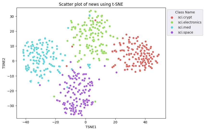
คุณจะใช้วิธีการฝังแบบ t-Distributd Stochastic Neighbor embedding (t-SNE) เพื่อลดมิติข้อมูล เทคนิคนี้จะช่วยลดจํานวนมิติข้อมูล ในขณะที่คงคลัสเตอร์ไว้ (จุดที่อยู่ใกล้กันจะยังอยู่ใกล้กัน) สำหรับข้อมูลเดิม โมเดลจะพยายามสร้างการกระจายที่จุดข้อมูลอื่นๆ เป็น "เพื่อนบ้าน" (เช่น ข้อมูลทั้งสองมีความหมายคล้ายกัน) จากนั้นจะเพิ่มประสิทธิภาพฟังก์ชันวัตถุประสงค์เพื่อให้มีการกระจายที่คล้ายกันในการแสดงภาพ

tsne = TSNE(random_state=0, n_iter=1000)
tsne_results = tsne.fit_transform(X)

df_tsne = pd.DataFrame(tsne_results, columns=['TSNE1', 'TSNE2'])
df_tsne['Class Name'] = df_train['Class Name'] # Add labels column from df_train to df_tsne
df_tsne

fig, ax = plt.subplots(figsize=(8,6)) # Set figsize
sns.set_style('darkgrid', {"grid.color": ".6", "grid.linestyle": ":"})
sns.scatterplot(data=df_tsne, x='TSNE1', y='TSNE2', hue='Class Name', palette='hls')
sns.move_legend(ax, "upper left", bbox_to_anchor=(1, 1))
plt.title('Scatter plot of news using t-SNE');
plt.xlabel('TSNE1');
plt.ylabel('TSNE2');
plt.axis('equal')

(-46.191162300109866,
 53.521015357971194,
 -39.96646995544434,
 37.282975387573245)

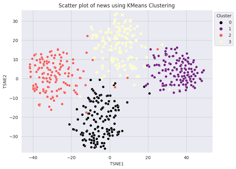
เปรียบเทียบผลลัพธ์กับ KMeans

คลัสเตอร์ KMeans เป็นอัลกอริทึมการจัดกลุ่มที่ได้รับความนิยมและใช้บ่อยสำหรับการเรียนรู้แบบไม่มีการควบคุมดูแล ซึ่งจะกำหนดจุดศูนย์กลางที่ดีที่สุดซ้ำๆ และกำหนดแต่ละตัวอย่างให้กับเซนทรอยด์ที่ใกล้ที่สุด ป้อนการฝังลงในอัลกอริทึม KMeans โดยตรงเพื่อเปรียบเทียบการแสดงภาพของการฝังกับประสิทธิภาพของอัลกอริทึมแมชชีนเลิร์นนิง

# Apply KMeans
kmeans_model = KMeans(n_clusters=4, random_state=1, n_init='auto').fit(X)
labels = kmeans_model.fit_predict(X)

df_tsne['Cluster'] = labels
df_tsne

fig, ax = plt.subplots(figsize=(8,6)) # Set figsize
sns.set_style('darkgrid', {"grid.color": ".6", "grid.linestyle": ":"})
sns.scatterplot(data=df_tsne, x='TSNE1', y='TSNE2', hue='Cluster', palette='magma')
sns.move_legend(ax, "upper left", bbox_to_anchor=(1, 1))
plt.title('Scatter plot of news using KMeans Clustering');
plt.xlabel('TSNE1');
plt.ylabel('TSNE2');
plt.axis('equal')

(-46.191162300109866,
 53.521015357971194,
 -39.96646995544434,
 37.282975387573245)

def get_majority_cluster_per_group(df_tsne_cluster, class_names):
  class_clusters = dict()
  for c in class_names:
    # Get rows of dataframe that are equal to c
    rows = df_tsne_cluster.loc[df_tsne_cluster['Class Name'] == c]
    # Get majority value in Cluster column of the rows selected
    cluster = rows.Cluster.mode().values[0]
    # Populate mapping dictionary
    class_clusters[c] = cluster
  return class_clusters

classes = df_tsne['Class Name'].unique()
class_clusters = get_majority_cluster_per_group(df_tsne, classes)
class_clusters

{'sci.crypt': 1, 'sci.electronics': 3, 'sci.med': 2, 'sci.space': 0}

รับคลัสเตอร์ส่วนใหญ่ต่อกลุ่ม และดูจำนวนสมาชิกจริงของกลุ่มนั้นที่อยู่ในคลัสเตอร์นั้น

# Convert the Cluster column to use the class name
class_by_id = {v: k for k, v in class_clusters.items()}
df_tsne['Predicted'] = df_tsne['Cluster'].map(class_by_id.__getitem__)

# Filter to the correctly matched rows
correct = df_tsne[df_tsne['Class Name'] == df_tsne['Predicted']]

# Summarise, as a percentage
acc = correct['Class Name'].value_counts() / SAMPLE_SIZE
acc

sci.space          0.966667
sci.med            0.960000
sci.electronics    0.953333
sci.crypt          0.926667
Name: Class Name, dtype: float64

# Get predicted values by name
df_tsne['Predicted'] = ''
for idx, rows in df_tsne.iterrows():
  cluster = rows['Cluster']
  # Get key from mapping based on cluster value
  key = list(class_clusters.keys())[list(class_clusters.values()).index(cluster)]
  df_tsne.at[idx, 'Predicted'] = key

df_tsne

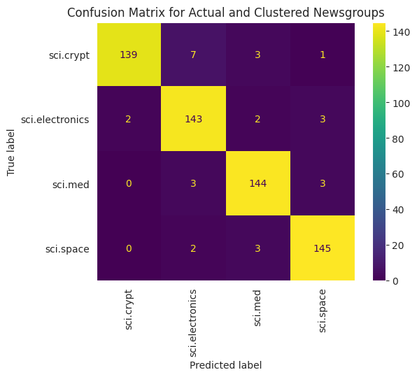
เพื่อให้เห็นภาพประสิทธิภาพของ KMeans ที่ใช้กับข้อมูลของคุณได้ดียิ่งขึ้น คุณสามารถใช้เมทริกซ์ความสับสน เมทริกซ์ความสับสนช่วยให้คุณประเมินประสิทธิภาพของโมเดลการจัดประเภทนอกเหนือจากความถูกต้อง คุณดูได้ว่าคะแนนที่จัดประเภทอย่างไม่ถูกต้องได้รับการจัดประเภทเป็นใดบ้าง คุณจะต้องใช้ค่าจริงและค่าที่คาดการณ์ ซึ่งได้รวบรวมไว้ในเฟรมข้อมูลด้านบน

cm = confusion_matrix(df_tsne['Class Name'].to_list(), df_tsne['Predicted'].to_list())
disp = ConfusionMatrixDisplay(confusion_matrix=cm,
                              display_labels=classes)
disp.plot(xticks_rotation='vertical')
plt.title('Confusion Matrix for Actual and Clustered Newsgroups');
plt.grid(False)

ขั้นตอนถัดไป

ต่อไปนี้คุณได้สร้างการแสดงภาพของการฝังด้วยคลัสเตอร์ของคุณเองแล้ว ลองใช้ข้อมูลที่เป็นข้อความของคุณเองเพื่อแสดงข้อความเหล่านั้นเป็นการฝัง คุณสามารถลดมิติข้อมูลเพื่อทำขั้นตอนการแสดงข้อมูลผ่านภาพให้เสร็จสิ้น โปรดทราบว่า TSNE นั้นดีในการจัดกลุ่มอินพุต แต่อาจใช้เวลานานขึ้นในการบรรจบกันหรืออาจติดอยู่ที่ค่าต่ำสุดในเครื่อง หากพบปัญหานี้ เทคนิคอีกอย่างที่คุณอาจลองใช้คือการวิเคราะห์องค์ประกอบหลัก (PCA)

นอกจากนี้ยังมีอัลกอริทึมการจัดกลุ่มอื่นๆ นอก KMeans ด้วยเช่นกัน เช่น การจัดคลัสเตอร์ตามความหนาแน่น (DBSCAN)

หากต้องการดูวิธีใช้บริการอื่นๆ ใน Gemini API ให้ไปที่การเริ่มต้นอย่างรวดเร็วสำหรับ Python หากต้องการเรียนรู้เพิ่มเติมเกี่ยวกับวิธีใช้การฝัง โปรดดูตัวอย่างที่มีอยู่ หากต้องการดูวิธีสร้างตั้งแต่ต้น โปรดดูบทแนะนำการฝังคำของ TensorFlow