
|
|
|
 Xem sổ tay trên GitHub Xem sổ tay trên GitHub
|
Tổng quan
Hướng dẫn này minh hoạ cách sử dụng các mục nhúng của Gemini API để phát hiện các điểm ngoại lai có thể xảy ra trong tập dữ liệu của bạn. Bạn sẽ mô phỏng trực quan một tập hợp con của tập dữ liệu 20 Newsgroup bằng cách sử dụng t-SNE và phát hiện các điểm ngoại lai bên ngoài một bán kính cụ thể của điểm trung tâm của mỗi cụm phân loại.
Để biết thêm thông tin về cách bắt đầu sử dụng các mục nhúng được tạo từ Gemini API, hãy xem tài liệu Bắt đầu nhanh về Python.
Điều kiện tiên quyết
Bạn có thể chạy quy trình bắt đầu nhanh này trong Google Colab.
Để hoàn thành quy trình bắt đầu nhanh này về môi trường phát triển của riêng bạn, hãy đảm bảo rằng môi trường của bạn đáp ứng các yêu cầu sau:
- Python 3.9 trở lên
- Cài đặt
jupyterđể chạy sổ tay.
Thiết lập
Trước tiên, hãy tải thư viện Gemini API Python xuống và cài đặt.
pip install -U -q google.generativeai
import re
import tqdm
import numpy as np
import pandas as pd
import matplotlib.pyplot as plt
import seaborn as sns

import google.generativeai as genai

# Used to securely store your API key
from google.colab import userdata

from sklearn.datasets import fetch_20newsgroups
from sklearn.manifold import TSNE
Lấy khoá API
Để có thể sử dụng Gemini API, trước tiên, bạn phải có khoá API. Nếu bạn chưa có khoá, hãy tạo khoá chỉ bằng một cú nhấp chuột trong Google AI Studio.
Trong Colab, hãy thêm khoá vào trình quản lý bí mật trong phần "🔑" trong bảng điều khiển bên trái. Đặt tên cho tệp đó là API_KEY.
Sau khi bạn có khoá API, hãy chuyển khoá đó vào SDK. Bạn có thể làm điều này theo hai cách:
- Đặt khoá vào biến môi trường
GOOGLE_API_KEY(SDK sẽ tự động nhận khoá từ đó). - Truyền khoá cho
genai.configure(api_key=...)
genai.configure(api_key=GOOGLE_API_KEY)
for m in genai.list_models():
  if 'embedContent' in m.supported_generation_methods:
    print(m.name)
models/embedding-001
models/embedding-001
Chuẩn bị tập dữ liệu
Tập dữ liệu văn bản 20 Newsgroups chứa 18.000 bài đăng của nhóm tin tức về 20 chủ đề được chia thành các tập huấn luyện và kiểm thử. Việc phân chia giữa tập dữ liệu huấn luyện và tập dữ liệu kiểm thử là dựa trên các thông báo được đăng trước và sau một ngày cụ thể. Hướng dẫn này sử dụng tập hợp con huấn luyện.
newsgroups_train = fetch_20newsgroups(subset='train')

# View list of class names for dataset
newsgroups_train.target_names
['alt.atheism',
 'comp.graphics',
 'comp.os.ms-windows.misc',
 'comp.sys.ibm.pc.hardware',
 'comp.sys.mac.hardware',
 'comp.windows.x',
 'misc.forsale',
 'rec.autos',
 'rec.motorcycles',
 'rec.sport.baseball',
 'rec.sport.hockey',
 'sci.crypt',
 'sci.electronics',
 'sci.med',
 'sci.space',
 'soc.religion.christian',
 'talk.politics.guns',
 'talk.politics.mideast',
 'talk.politics.misc',
 'talk.religion.misc']
Đây là ví dụ đầu tiên trong tập huấn luyện.
idx = newsgroups_train.data[0].index('Lines')
print(newsgroups_train.data[0][idx:])
Lines: 15

 I was wondering if anyone out there could enlighten me on this car I saw
the other day. It was a 2-door sports car, looked to be from the late 60s/
early 70s. It was called a Bricklin. The doors were really small. In addition,
the front bumper was separate from the rest of the body. This is
all I know. If anyone can tellme a model name, engine specs, years
of production, where this car is made, history, or whatever info you
have on this funky looking car, please e-mail.

Thanks,

- IL
   ---- brought to you by your neighborhood Lerxst ----
# Apply functions to remove names, emails, and extraneous words from data points in newsgroups.data
newsgroups_train.data = [re.sub(r'[\w\.-]+@[\w\.-]+', '', d) for d in newsgroups_train.data] # Remove email
newsgroups_train.data = [re.sub(r"\([^()]*\)", "", d) for d in newsgroups_train.data] # Remove names
newsgroups_train.data = [d.replace("From: ", "") for d in newsgroups_train.data] # Remove "From: "
newsgroups_train.data = [d.replace("\nSubject: ", "") for d in newsgroups_train.data] # Remove "\nSubject: "

# Cut off each text entry after 5,000 characters
newsgroups_train.data = [d[0:5000] if len(d) > 5000 else d for d in newsgroups_train.data]
# Put training points into a dataframe
df_train = pd.DataFrame(newsgroups_train.data, columns=['Text'])
df_train['Label'] = newsgroups_train.target
# Match label to target name index
df_train['Class Name'] = df_train['Label'].map(newsgroups_train.target_names.__getitem__)

df_train
Tiếp theo, hãy lấy mẫu một số dữ liệu bằng cách lấy 150 điểm dữ liệu trong tập dữ liệu huấn luyện rồi chọn một vài danh mục. Hướng dẫn này sử dụng các danh mục khoa học.
# Take a sample of each label category from df_train
SAMPLE_SIZE = 150
df_train = (df_train.groupby('Label', as_index = False)
                    .apply(lambda x: x.sample(SAMPLE_SIZE))
                    .reset_index(drop=True))

# Choose categories about science
df_train = df_train[df_train['Class Name'].str.contains('sci')]

# Reset the index
df_train = df_train.reset_index()
df_train
df_train['Class Name'].value_counts()
sci.crypt          150
sci.electronics    150
sci.med            150
sci.space          150
Name: Class Name, dtype: int64
Tạo các mục nhúng
Trong phần này, bạn sẽ tìm hiểu cách tạo các mục nhúng cho các văn bản khác nhau trong khung dữ liệu bằng cách sử dụng các mục nhúng từ Gemini API.
Thay đổi về API đối với mục Nhúng với mô hình nhúng-001
Đối với mô hình nhúng mới, Nhúng-001, có một tham số loại tác vụ mới và tiêu đề không bắt buộc (chỉ hợp lệ với task_type=RETRIEVAL_DOCUMENT).
Các tham số mới này chỉ áp dụng cho các mô hình nhúng mới nhất.Có các loại tác vụ sau:
| Loại việc cần làm | Mô tả |
|---|---|
| RETRIEVAL_QUERY | Chỉ định văn bản đã cho là một truy vấn trong chế độ cài đặt tìm kiếm/truy xuất. |
| RETRIEVAL_DOCUMENT | Chỉ định văn bản đã cho là một tài liệu trong chế độ cài đặt tìm kiếm/truy xuất. |
| SEMANTIC_SIMILARITY | Cho biết văn bản đã cho sẽ được dùng để xác định tính tương đồng về mặt văn bản theo ngữ nghĩa (STS). |
| PHÂN LOẠI | Cho biết các mục nhúng sẽ được dùng để phân loại. |
| PHÂN TÍCH | Chỉ định xem các mục nhúng có được dùng để phân cụm hay không. |
from tqdm.auto import tqdm
tqdm.pandas()

from google.api_core import retry

def make_embed_text_fn(model):

  @retry.Retry(timeout=300.0)
  def embed_fn(text: str) -> list[float]:
    # Set the task_type to CLUSTERING.
    embedding = genai.embed_content(model=model,
                                    content=text,
                                    task_type="clustering")['embedding']
    return np.array(embedding)

  return embed_fn

def create_embeddings(df):
  model = 'models/embedding-001'
  df['Embeddings'] = df['Text'].progress_apply(make_embed_text_fn(model))
  return df

df_train = create_embeddings(df_train)
df_train.drop('index', axis=1, inplace=True)
0%| | 0/600 [00:00<?, ?it/s]
Giảm kích thước
Kích thước của vectơ nhúng tài liệu là 768. Để hình dung cách các tài liệu được nhúng được nhóm lại với nhau, bạn sẽ cần áp dụng tính năng giảm kích thước vì bạn chỉ có thể trực quan hoá các mục nhúng trong không gian 2D hoặc 3D. Các tài liệu tương tự về ngữ cảnh nên được đặt gần nhau hơn trong không gian thay vì các tài liệu không giống nhau.
len(df_train['Embeddings'][0])
768
# Convert df_train['Embeddings'] Pandas series to a np.array of float32
X = np.array(df_train['Embeddings'].to_list(), dtype=np.float32)
X.shape
(600, 768)
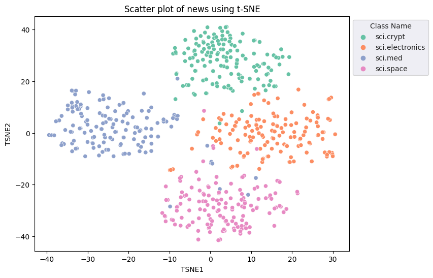
Bạn sẽ áp dụng phương pháp Nhúng lân cận Stochastic phân phối (t-SNE) để thực hiện việc giảm kích thước. Kỹ thuật này làm giảm số lượng phương diện, trong khi vẫn duy trì các cụm (các điểm gần nhau thì nằm gần nhau). Đối với dữ liệu gốc, mô hình này cố gắng xây dựng phân phối mà theo đó các điểm dữ liệu khác là "lân cận" (ví dụ: các từ khoá có ý nghĩa tương tự nhau). Sau đó, công cụ này tối ưu hoá một hàm mục tiêu để duy trì mức phân phối tương tự trong hình ảnh trực quan.
tsne = TSNE(random_state=0, n_iter=1000)
tsne_results = tsne.fit_transform(X)
df_tsne = pd.DataFrame(tsne_results, columns=['TSNE1', 'TSNE2'])
df_tsne['Class Name'] = df_train['Class Name'] # Add labels column from df_train to df_tsne
df_tsne
fig, ax = plt.subplots(figsize=(8,6)) # Set figsize
sns.set_style('darkgrid', {"grid.color": ".6", "grid.linestyle": ":"})
sns.scatterplot(data=df_tsne, x='TSNE1', y='TSNE2', hue='Class Name', palette='Set2')
sns.move_legend(ax, "upper left", bbox_to_anchor=(1, 1))
plt.title('Scatter plot of news using t-SNE')
plt.xlabel('TSNE1')
plt.ylabel('TSNE2');
Phát hiện điểm ngoại lai
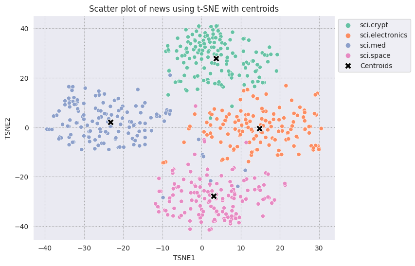
Để xác định điểm nào là điểm bất thường, bạn sẽ xác định điểm nào là điểm ngoại lai và điểm ngoại lai. Bắt đầu bằng cách tìm tâm hoặc vị trí đại diện cho tâm của cụm và sử dụng khoảng cách để xác định các điểm ngoại lai.
Hãy bắt đầu bằng cách lấy trọng tâm của từng danh mục.
def get_centroids(df_tsne):
  # Get the centroid of each cluster
  centroids = df_tsne.groupby('Class Name').mean()
  return centroids

centroids = get_centroids(df_tsne)
centroids
def get_embedding_centroids(df):
  emb_centroids = dict()
  grouped = df.groupby('Class Name')
  for c in grouped.groups:
    sub_df = grouped.get_group(c)
    # Get the centroid value of dimension 768
    emb_centroids[c] = np.mean(sub_df['Embeddings'], axis=0)

  return emb_centroids
emb_c = get_embedding_centroids(df_train)
Vẽ từng tâm bạn tìm được so với các điểm còn lại.
# Plot the centroids against the cluster
fig, ax = plt.subplots(figsize=(8,6)) # Set figsize
sns.set_style('darkgrid', {"grid.color": ".6", "grid.linestyle": ":"})
sns.scatterplot(data=df_tsne, x='TSNE1', y='TSNE2', hue='Class Name', palette='Set2');
sns.scatterplot(data=centroids, x='TSNE1', y='TSNE2', color="black", marker='X', s=100, label='Centroids')
sns.move_legend(ax, "upper left", bbox_to_anchor=(1, 1))
plt.title('Scatter plot of news using t-SNE with centroids')
plt.xlabel('TSNE1')
plt.ylabel('TSNE2');
Chọn một bán kính. Bất kỳ điều gì vượt quá giới hạn này từ trọng tâm của danh mục đó được coi là ngoại lệ.
def calculate_euclidean_distance(p1, p2):
  return np.sqrt(np.sum(np.square(p1 - p2)))

def detect_outlier(df, emb_centroids, radius):
  for idx, row in df.iterrows():
    class_name = row['Class Name'] # Get class name of row
    # Compare centroid distances
    dist = calculate_euclidean_distance(row['Embeddings'],
                                        emb_centroids[class_name])
    df.at[idx, 'Outlier'] = dist > radius

  return len(df[df['Outlier'] == True])
range_ = np.arange(0.3, 0.75, 0.02).round(decimals=2).tolist()
num_outliers = []
for i in range_:
  num_outliers.append(detect_outlier(df_train, emb_c, i))
# Plot range_ and num_outliers
fig = plt.figure(figsize = (14, 8))
plt.rcParams.update({'font.size': 12})
plt.bar(list(map(str, range_)), num_outliers)
plt.title("Number of outliers vs. distance of points from centroid")
plt.xlabel("Distance")
plt.ylabel("Number of outliers")
for i in range(len(range_)):
  plt.text(i, num_outliers[i], num_outliers[i], ha = 'center')

plt.show()
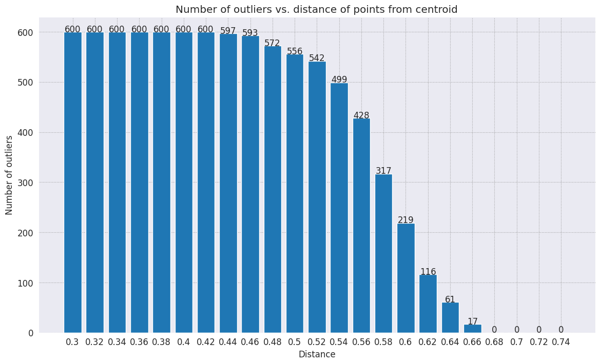
Tùy thuộc vào độ nhạy mà bạn muốn cho trình phát hiện hoạt động bất thường, bạn có thể chọn bán kính mình muốn sử dụng. Hiện tại, 0,62 được sử dụng, nhưng bạn có thể thay đổi giá trị này.
# View the points that are outliers
RADIUS = 0.62
detect_outlier(df_train, emb_c, RADIUS)
df_outliers = df_train[df_train['Outlier'] == True]
df_outliers.head()
# Use the index to map the outlier points back to the projected TSNE points
outliers_projected = df_tsne.loc[df_outliers['Outlier'].index]
Vẽ các điểm ngoại lai và biểu thị chúng bằng màu đỏ trong suốt.
fig, ax = plt.subplots(figsize=(8,6)) # Set figsize
plt.rcParams.update({'font.size': 10})
sns.set_style('darkgrid', {"grid.color": ".6", "grid.linestyle": ":"})
sns.scatterplot(data=df_tsne, x='TSNE1', y='TSNE2', hue='Class Name', palette='Set2');
sns.scatterplot(data=centroids, x='TSNE1', y='TSNE2', color="black", marker='X', s=100, label='Centroids')
# Draw a red circle around the outliers
sns.scatterplot(data=outliers_projected, x='TSNE1', y='TSNE2', color='red', marker='o', alpha=0.5, s=90, label='Outliers')
sns.move_legend(ax, "upper left", bbox_to_anchor=(1, 1))
plt.title('Scatter plot of news with outliers projected with t-SNE')
plt.xlabel('TSNE1')
plt.ylabel('TSNE2');
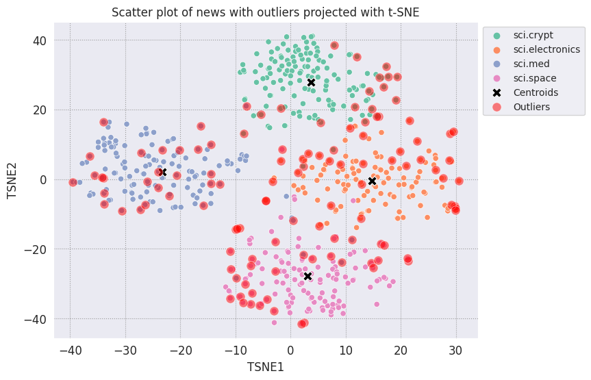
Sử dụng các giá trị chỉ mục của danh mục dữ liệu để in ra một vài ví dụ về các điểm ngoại lai có thể trông như thế nào trong mỗi danh mục. Tại đây, điểm dữ liệu đầu tiên từ mỗi danh mục sẽ được in. Khám phá các điểm khác trong từng danh mục để xem dữ liệu được coi là điểm bất thường hoặc điểm bất thường.
sci_crypt_outliers = df_outliers[df_outliers['Class Name'] == 'sci.crypt']
print(sci_crypt_outliers['Text'].iloc[0])
Re: Source of random bits on a Unix workstation
Lines: 44
Nntp-Posting-Host: sandstorm

>>For your application, what you can do is to encrypt the real-time clock
>>value with a secret key.

Well, almost.... If I only had to solve the problem for myself, and were
willing to have to type in a second password  whenever I
logged in, it could work. However, I'm trying to create a solution that
anyone can use, and which, once installed, is just as effortless to start up
as the non-solution of just using xhost to control access. I've got
religeous problems with storing secret keys on multiuser computers.

>For a good discussion of cryptographically "good" random number
>generators, check out the draft-ietf-security-randomness-00.txt
>Internet Draft, available at your local friendly internet drafts
>repository.

Thanks for the pointer! It was good reading, and I liked the idea of using
several unrelated sources with a strong mixing function. However, unless I
missed something, the only source they suggested
that seems available, and unguessable by an intruder, when a Unix is
fresh-booted, is I/O buffers related to network traffic. I believe my
solution basically uses that strategy, without requiring me to reach into
the kernel.

>A reasonably source of randomness is the output of a cryptographic
>hash function , when fed with a large amount of
>more-or-less random data. For example, running MD5 on /dev/mem is a
>slow, but random enough, source of random bits; there are bound to be
>128 bits of entropy in the tens  of megabytes of data in
>a modern workstation's memory, as a fair amount of them are system
>timers, i/o buffers, etc.

I heard about this solution, and it sounded good. Then I heard that folks
were experiencing times of 30-60 seconds to run this, on
reasonably-configured workstations. I'm not willing to add that much delay
to someone's login process. My approach  takes
a second or two to run. I'm considering writing the be-all and end-all of
solutions, that launches the MD5, and simultaneously tries to suck bits off
the net, and if the net should be sitting __SO__ idle that it can't get 10K
after compression before MD5 finishes, use the MD5. This way I could have
guaranteed good bits, and a deterministic upper bound on login time, and
still have the common case of login take only a couple of extra seconds.

-Bennett
sci_elec_outliers = df_outliers[df_outliers['Class Name'] == 'sci.electronics']
print(sci_elec_outliers['Text'].iloc[0])
Re: Laser vs Bubblejet?
Reply-To:
Distribution: world
X-Mailer: cppnews \\(Revision: 1.20 \\)
Organization: null
Lines: 53

Here is a different viewpoint.

> FYI:  The actual horizontal dot placement resoution of an HP
> deskjet is 1/600th inch.  The electronics and dynamics of the ink
> cartridge, however, limit you to generating dots at 300 per inch.
> On almost any paper, the ink wicks more than 1/300th inch anyway.
>
> The method of depositing and fusing toner of a laster printer
> results in much less spread than ink drop technology.

In practice there is little difference in quality but more care is needed
with inkjet because smudges etc. can happen.

> It doesn't take much investigation to see that the mechanical and
> electronic complement of a laser printer is more complex than
> inexpensive ink jet printers.  Recall also that laser printers
> offer a much higher throughput:  10 ppm for a laser versus about 1
> ppm for an ink jet printer.

A cheap laser printer does not manage that sort of throughput and on top of
that how long does the _first_ sheet take to print? Inkjets are faster than
you say and in both cases the computer often has trouble keeping up with the
printer.

A sage said to me: "Do you want one copy or lots of copies?", "One",
"Inkjet".

> Something else to think about is the cost of consumables over the
> life of the printer.  A 3000 page yield toner cartridge is about
> $US 75-80 at discount while HP high capacity
> cartridges are about $US 22 at discount.  It could be that over the
> life cycle of the printer that consumables for laser printers are
> less than ink jet printers.  It is getting progressively closer
> between the two technologies.  Laser printers are usually desinged
> for higher duty cycles in pages per month and longer product
> replacement cycles.

Paper cost is the same and both can use refills. Long term the laserprinter
will need some expensive replacement parts  and on top of that
are the amortisation costs which favour the lowest purchase cost printer.

HP inkjets understand PCL so in many cases a laserjet driver will work if the
software package has no inkjet driver.

There is one wild difference between the two printers: a laserprinter is a
page printer whilst an inkjet is a line printer. This means that a
laserprinter can rotate graphic images whilst an inkjet cannot. Few drivers
actually use this facility.


  TC.
    E-mail:  or
sci_med_outliers = df_outliers[df_outliers['Class Name'] == 'sci.med']
print(sci_med_outliers['Text'].iloc[0])
Re: THE BACK MACHINE - Update
Organization: University of Nebraska--Lincoln
Lines: 15
Distribution: na
NNTP-Posting-Host: unlinfo.unl.edu

   I have a BACK MACHINE and have had one since January.  While I have not
found it to be a panacea for my back pain, I think it has helped somewhat.
It MAINLY acts to stretch muscles in the back and prevent spasms associated
with pain.  I am taking less pain medication than I was previously.
   The folks at BACK TECHNOLOGIES are VERY reluctant to honor their return
policy.  They extended my "warranty" period rather than allow me to return
the machine when, after the first month or so, I was not thrilled with it.
They encouraged me to continue to use it, abeit less vigourously.
   Like I said, I can't say it is a cure-all, but it keeps me stretched out
and I am in less pain.
--
***********************************************************************
Dale M. Webb, DVM, PhD           *  97% of the body is water.  The
Veterinary Diagnostic Center     *  other 3% keeps you from drowning.
University of Nebraska, Lincoln  *
sci_space_outliers = df_outliers[df_outliers['Class Name'] == 'sci.space']
print(sci_space_outliers['Text'].iloc[0])
MACH 25 landing site bases?
Article-I.D.: aurora.1993Apr5.193829.1
Organization: University of Alaska Fairbanks
Lines: 7
Nntp-Posting-Host: acad3.alaska.edu

The supersonic booms hear a few months ago over I belive San Fran, heading east
of what I heard, some new super speed Mach 25 aircraft?? What military based
int he direction of flight are there that could handle a Mach 25aircraft on its
landing decent?? Odd question??

==
Michael Adams,  -- I'm not high, just jacked
Các bước tiếp theo
Giờ đây, bạn đã tạo được trình phát hiện hoạt động bất thường bằng cách sử dụng các mục nhúng! Hãy thử sử dụng dữ liệu văn bản của riêng bạn để trực quan hoá chúng dưới dạng các tệp nhúng và chọn một số ràng buộc sao cho có thể phát hiện các điểm ngoại lai. Bạn có thể giảm kích thước để hoàn tất bước tạo hình ảnh trực quan. Lưu ý rằng t-SNE rất hiệu quả trong việc phân cụm đầu vào, nhưng có thể mất nhiều thời gian hơn để hội tụ hoặc có thể bị kẹt ở mức tối thiểu cục bộ. Nếu gặp vấn đề này, bạn có thể cân nhắc sử dụng một kỹ thuật khác là phân tích các thành phần chính (PCA).
Để tìm hiểu thêm về cách sử dụng tính năng nhúng, hãy xem các hướng dẫn khác sau đây: