
|
|
|
 Visualizza blocco note su GitHub Visualizza blocco note su GitHub
|
Panoramica
Questo tutorial mostra come utilizzare gli incorporamenti dell'API Gemini per rilevare potenziali outlier nel set di dati. Vedrai un sottoinsieme del set di dati dei 20 Newsgroup utilizzando t-SNE e rileverai gli outlier al di fuori di un determinato raggio del punto centrale di ciascun cluster categorico.
Per saperne di più su come iniziare a utilizzare gli incorporamenti generati dall'API Gemini, consulta la guida rapida di Python.
Prerequisiti
Puoi eseguire questa guida rapida in Google Colab.
Per completare questa guida rapida nel tuo ambiente di sviluppo, assicurati che l'ambiente soddisfi i seguenti requisiti:
- Python 3.9 o versioni successive
- Un'installazione di
jupyterper eseguire il blocco note.
Configurazione
Innanzitutto, scarica e installa la libreria Python dell'API Gemini.
pip install -U -q google.generativeai
import re
import tqdm
import numpy as np
import pandas as pd
import matplotlib.pyplot as plt
import seaborn as sns

import google.generativeai as genai

# Used to securely store your API key
from google.colab import userdata

from sklearn.datasets import fetch_20newsgroups
from sklearn.manifold import TSNE
Procurati una chiave API
Prima di poter utilizzare l'API Gemini, devi ottenere una chiave API. Se non ne hai già una, crea una chiave con un solo clic in Google AI Studio.
In Colab, aggiungi la chiave a Secret Manager nella sezione " {/8}" nel riquadro a sinistra. Assegnagli il nome API_KEY.
Una volta ottenuta la chiave API, passala all'SDK. A tale scopo, puoi procedere in uno dei due seguenti modi:
- Inserisci la chiave nella variabile di ambiente
GOOGLE_API_KEY(l'SDK la acquisirà automaticamente da lì). - Passa la chiave a
genai.configure(api_key=...)
genai.configure(api_key=GOOGLE_API_KEY)
for m in genai.list_models():
  if 'embedContent' in m.supported_generation_methods:
    print(m.name)
models/embedding-001
models/embedding-001
Prepara il set di dati
Il set di dati di testo 20 Newsgroups contiene 18.000 post di newsgroup su 20 argomenti,suddivisi in set di addestramento e test. La suddivisione tra i set di dati di addestramento e test si basa sui messaggi pubblicati prima e dopo una data specifica. Questo tutorial utilizza il sottoinsieme di addestramento.
newsgroups_train = fetch_20newsgroups(subset='train')

# View list of class names for dataset
newsgroups_train.target_names
['alt.atheism',
 'comp.graphics',
 'comp.os.ms-windows.misc',
 'comp.sys.ibm.pc.hardware',
 'comp.sys.mac.hardware',
 'comp.windows.x',
 'misc.forsale',
 'rec.autos',
 'rec.motorcycles',
 'rec.sport.baseball',
 'rec.sport.hockey',
 'sci.crypt',
 'sci.electronics',
 'sci.med',
 'sci.space',
 'soc.religion.christian',
 'talk.politics.guns',
 'talk.politics.mideast',
 'talk.politics.misc',
 'talk.religion.misc']
Ecco il primo esempio del set di addestramento.
idx = newsgroups_train.data[0].index('Lines')
print(newsgroups_train.data[0][idx:])
Lines: 15

 I was wondering if anyone out there could enlighten me on this car I saw
the other day. It was a 2-door sports car, looked to be from the late 60s/
early 70s. It was called a Bricklin. The doors were really small. In addition,
the front bumper was separate from the rest of the body. This is
all I know. If anyone can tellme a model name, engine specs, years
of production, where this car is made, history, or whatever info you
have on this funky looking car, please e-mail.

Thanks,

- IL
   ---- brought to you by your neighborhood Lerxst ----
# Apply functions to remove names, emails, and extraneous words from data points in newsgroups.data
newsgroups_train.data = [re.sub(r'[\w\.-]+@[\w\.-]+', '', d) for d in newsgroups_train.data] # Remove email
newsgroups_train.data = [re.sub(r"\([^()]*\)", "", d) for d in newsgroups_train.data] # Remove names
newsgroups_train.data = [d.replace("From: ", "") for d in newsgroups_train.data] # Remove "From: "
newsgroups_train.data = [d.replace("\nSubject: ", "") for d in newsgroups_train.data] # Remove "\nSubject: "

# Cut off each text entry after 5,000 characters
newsgroups_train.data = [d[0:5000] if len(d) > 5000 else d for d in newsgroups_train.data]
# Put training points into a dataframe
df_train = pd.DataFrame(newsgroups_train.data, columns=['Text'])
df_train['Label'] = newsgroups_train.target
# Match label to target name index
df_train['Class Name'] = df_train['Label'].map(newsgroups_train.target_names.__getitem__)

df_train
Poi, campiona alcuni dati prendendo 150 punti dati nel set di dati di addestramento e scegliendo alcune categorie. Questo tutorial utilizza le categorie scientifiche.
# Take a sample of each label category from df_train
SAMPLE_SIZE = 150
df_train = (df_train.groupby('Label', as_index = False)
                    .apply(lambda x: x.sample(SAMPLE_SIZE))
                    .reset_index(drop=True))

# Choose categories about science
df_train = df_train[df_train['Class Name'].str.contains('sci')]

# Reset the index
df_train = df_train.reset_index()
df_train
df_train['Class Name'].value_counts()
sci.crypt          150
sci.electronics    150
sci.med            150
sci.space          150
Name: Class Name, dtype: int64
Crea gli incorporamenti
In questa sezione, vedrai come generare incorporamenti per i diversi testi nel dataframe utilizzando gli incorporamenti dell'API Gemini.
Modifiche all'API per gli incorporamenti con il modello Embedding-001
Per il nuovo modello degli incorporamenti, Embedding-001, sono disponibili un nuovo parametro per il tipo di attività e il titolo facoltativo (valido solo con task_type=RETRIEVAL_DOCUMENT).
Questi nuovi parametri si applicano solo ai modelli di incorporamenti più recenti.I tipi di attività sono:
| Tipo di attività | Descrizione |
|---|---|
| RETRIEVAL_QUERY | Specifica che il testo specificato è una query in un'impostazione di ricerca/recupero. |
| RETRIEVAL_DOCUMENT | Specifica che il testo specificato è un documento in un'impostazione di ricerca/recupero. |
| SEMANTIC_SIMILARITY | Specifica il testo specificato che verrà utilizzato per la somiglianza testuale semantica (STS). |
| CLASSIFICAZIONE | Specifica che gli incorporamenti verranno utilizzati per la classificazione. |
| CLUSTERING | Specifica che gli incorporamenti verranno utilizzati per il clustering. |
from tqdm.auto import tqdm
tqdm.pandas()

from google.api_core import retry

def make_embed_text_fn(model):

  @retry.Retry(timeout=300.0)
  def embed_fn(text: str) -> list[float]:
    # Set the task_type to CLUSTERING.
    embedding = genai.embed_content(model=model,
                                    content=text,
                                    task_type="clustering")['embedding']
    return np.array(embedding)

  return embed_fn

def create_embeddings(df):
  model = 'models/embedding-001'
  df['Embeddings'] = df['Text'].progress_apply(make_embed_text_fn(model))
  return df

df_train = create_embeddings(df_train)
df_train.drop('index', axis=1, inplace=True)
0%| | 0/600 [00:00<?, ?it/s]
Riduzione della dimensionalità
La dimensione del vettore di incorporamento del documento è 768. Per visualizzare come vengono raggruppati i documenti incorporati, dovrai applicare la riduzione della dimensionalità, poiché puoi visualizzare gli incorporamenti solo in uno spazio 2D o 3D. I documenti contestualimente simili dovrebbero essere più vicini nello spazio rispetto a documenti meno simili.
len(df_train['Embeddings'][0])
768
# Convert df_train['Embeddings'] Pandas series to a np.array of float32
X = np.array(df_train['Embeddings'].to_list(), dtype=np.float32)
X.shape
(600, 768)
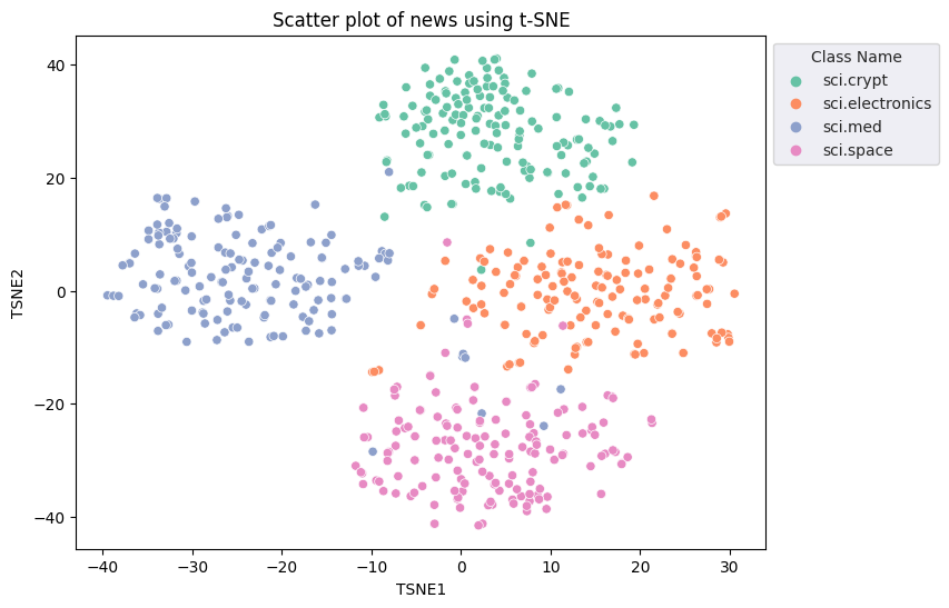
Applicherai l'approccio t-Distributed Stochastic Nearby Embedding (t-SNE) per ridurre la dimensionalità. Questa tecnica riduce il numero di dimensioni, conservando i cluster (i punti vicini rimangono vicini). Per i dati originali, il modello cerca di costruire una distribuzione di cui gli altri punti dati siano "vicini" (ad es. hanno un significato simile). Ottimizza quindi una funzione obiettivo per mantenere una distribuzione simile nella visualizzazione.
tsne = TSNE(random_state=0, n_iter=1000)
tsne_results = tsne.fit_transform(X)
df_tsne = pd.DataFrame(tsne_results, columns=['TSNE1', 'TSNE2'])
df_tsne['Class Name'] = df_train['Class Name'] # Add labels column from df_train to df_tsne
df_tsne
fig, ax = plt.subplots(figsize=(8,6)) # Set figsize
sns.set_style('darkgrid', {"grid.color": ".6", "grid.linestyle": ":"})
sns.scatterplot(data=df_tsne, x='TSNE1', y='TSNE2', hue='Class Name', palette='Set2')
sns.move_legend(ax, "upper left", bbox_to_anchor=(1, 1))
plt.title('Scatter plot of news using t-SNE')
plt.xlabel('TSNE1')
plt.ylabel('TSNE2');
Rilevamento outlier
Per determinare quali punti sono anomali, dovrai stabilire quali sono i punti intenzionali e anomali. Inizia individuando il centroide o la posizione che rappresenta il centro del cluster e utilizza la distanza per determinare i punti che sono outlier.
Per iniziare, ottieni il centroide di ogni categoria.
def get_centroids(df_tsne):
  # Get the centroid of each cluster
  centroids = df_tsne.groupby('Class Name').mean()
  return centroids

centroids = get_centroids(df_tsne)
centroids
def get_embedding_centroids(df):
  emb_centroids = dict()
  grouped = df.groupby('Class Name')
  for c in grouped.groups:
    sub_df = grouped.get_group(c)
    # Get the centroid value of dimension 768
    emb_centroids[c] = np.mean(sub_df['Embeddings'], axis=0)

  return emb_centroids
emb_c = get_embedding_centroids(df_train)
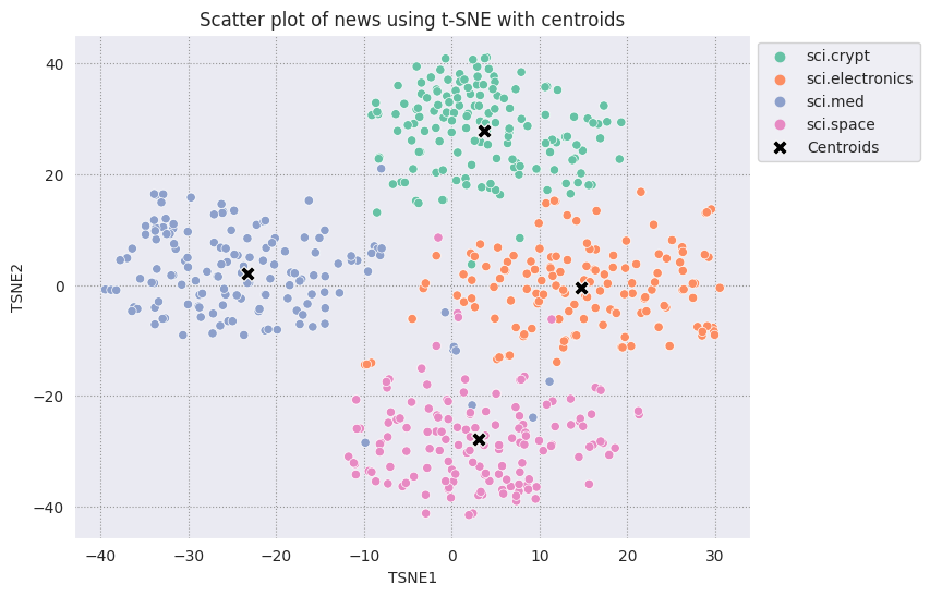
Traccia ciascun centroide trovato rispetto agli altri punti.
# Plot the centroids against the cluster
fig, ax = plt.subplots(figsize=(8,6)) # Set figsize
sns.set_style('darkgrid', {"grid.color": ".6", "grid.linestyle": ":"})
sns.scatterplot(data=df_tsne, x='TSNE1', y='TSNE2', hue='Class Name', palette='Set2');
sns.scatterplot(data=centroids, x='TSNE1', y='TSNE2', color="black", marker='X', s=100, label='Centroids')
sns.move_legend(ax, "upper left", bbox_to_anchor=(1, 1))
plt.title('Scatter plot of news using t-SNE with centroids')
plt.xlabel('TSNE1')
plt.ylabel('TSNE2');
Scegli un raggio. Qualsiasi elemento al di fuori di questo limite dal centroide di quella categoria è considerato un outlier.
def calculate_euclidean_distance(p1, p2):
  return np.sqrt(np.sum(np.square(p1 - p2)))

def detect_outlier(df, emb_centroids, radius):
  for idx, row in df.iterrows():
    class_name = row['Class Name'] # Get class name of row
    # Compare centroid distances
    dist = calculate_euclidean_distance(row['Embeddings'],
                                        emb_centroids[class_name])
    df.at[idx, 'Outlier'] = dist > radius

  return len(df[df['Outlier'] == True])
range_ = np.arange(0.3, 0.75, 0.02).round(decimals=2).tolist()
num_outliers = []
for i in range_:
  num_outliers.append(detect_outlier(df_train, emb_c, i))
# Plot range_ and num_outliers
fig = plt.figure(figsize = (14, 8))
plt.rcParams.update({'font.size': 12})
plt.bar(list(map(str, range_)), num_outliers)
plt.title("Number of outliers vs. distance of points from centroid")
plt.xlabel("Distance")
plt.ylabel("Number of outliers")
for i in range(len(range_)):
  plt.text(i, num_outliers[i], num_outliers[i], ha = 'center')

plt.show()
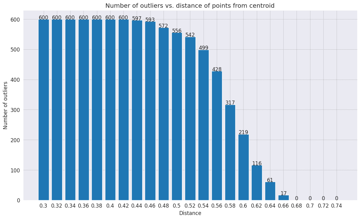
A seconda di quanto vuoi che sia sensibile il rilevatore di anomalie, puoi scegliere il raggio da utilizzare. Per ora, viene usato 0,62, ma puoi modificare questo valore.
# View the points that are outliers
RADIUS = 0.62
detect_outlier(df_train, emb_c, RADIUS)
df_outliers = df_train[df_train['Outlier'] == True]
df_outliers.head()
# Use the index to map the outlier points back to the projected TSNE points
outliers_projected = df_tsne.loc[df_outliers['Outlier'].index]
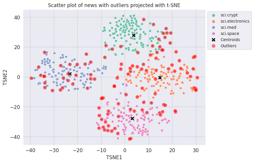
Traccia i valori anomali e indicali con un colore rosso trasparente.
fig, ax = plt.subplots(figsize=(8,6)) # Set figsize
plt.rcParams.update({'font.size': 10})
sns.set_style('darkgrid', {"grid.color": ".6", "grid.linestyle": ":"})
sns.scatterplot(data=df_tsne, x='TSNE1', y='TSNE2', hue='Class Name', palette='Set2');
sns.scatterplot(data=centroids, x='TSNE1', y='TSNE2', color="black", marker='X', s=100, label='Centroids')
# Draw a red circle around the outliers
sns.scatterplot(data=outliers_projected, x='TSNE1', y='TSNE2', color='red', marker='o', alpha=0.5, s=90, label='Outliers')
sns.move_legend(ax, "upper left", bbox_to_anchor=(1, 1))
plt.title('Scatter plot of news with outliers projected with t-SNE')
plt.xlabel('TSNE1')
plt.ylabel('TSNE2');
Utilizza i valori di indice dei datafame per stampare alcuni esempi di come possono apparire i valori anomali in ciascuna categoria. Qui viene stampato il primo punto dati di ogni categoria. Esplora altri punti in ogni categoria per visualizzare i dati considerati come outlier o anomalie.
sci_crypt_outliers = df_outliers[df_outliers['Class Name'] == 'sci.crypt']
print(sci_crypt_outliers['Text'].iloc[0])
Re: Source of random bits on a Unix workstation
Lines: 44
Nntp-Posting-Host: sandstorm

>>For your application, what you can do is to encrypt the real-time clock
>>value with a secret key.

Well, almost.... If I only had to solve the problem for myself, and were
willing to have to type in a second password  whenever I
logged in, it could work. However, I'm trying to create a solution that
anyone can use, and which, once installed, is just as effortless to start up
as the non-solution of just using xhost to control access. I've got
religeous problems with storing secret keys on multiuser computers.

>For a good discussion of cryptographically "good" random number
>generators, check out the draft-ietf-security-randomness-00.txt
>Internet Draft, available at your local friendly internet drafts
>repository.

Thanks for the pointer! It was good reading, and I liked the idea of using
several unrelated sources with a strong mixing function. However, unless I
missed something, the only source they suggested
that seems available, and unguessable by an intruder, when a Unix is
fresh-booted, is I/O buffers related to network traffic. I believe my
solution basically uses that strategy, without requiring me to reach into
the kernel.

>A reasonably source of randomness is the output of a cryptographic
>hash function , when fed with a large amount of
>more-or-less random data. For example, running MD5 on /dev/mem is a
>slow, but random enough, source of random bits; there are bound to be
>128 bits of entropy in the tens  of megabytes of data in
>a modern workstation's memory, as a fair amount of them are system
>timers, i/o buffers, etc.

I heard about this solution, and it sounded good. Then I heard that folks
were experiencing times of 30-60 seconds to run this, on
reasonably-configured workstations. I'm not willing to add that much delay
to someone's login process. My approach  takes
a second or two to run. I'm considering writing the be-all and end-all of
solutions, that launches the MD5, and simultaneously tries to suck bits off
the net, and if the net should be sitting __SO__ idle that it can't get 10K
after compression before MD5 finishes, use the MD5. This way I could have
guaranteed good bits, and a deterministic upper bound on login time, and
still have the common case of login take only a couple of extra seconds.

-Bennett
sci_elec_outliers = df_outliers[df_outliers['Class Name'] == 'sci.electronics']
print(sci_elec_outliers['Text'].iloc[0])
Re: Laser vs Bubblejet?
Reply-To:
Distribution: world
X-Mailer: cppnews \\(Revision: 1.20 \\)
Organization: null
Lines: 53

Here is a different viewpoint.

> FYI:  The actual horizontal dot placement resoution of an HP
> deskjet is 1/600th inch.  The electronics and dynamics of the ink
> cartridge, however, limit you to generating dots at 300 per inch.
> On almost any paper, the ink wicks more than 1/300th inch anyway.
>
> The method of depositing and fusing toner of a laster printer
> results in much less spread than ink drop technology.

In practice there is little difference in quality but more care is needed
with inkjet because smudges etc. can happen.

> It doesn't take much investigation to see that the mechanical and
> electronic complement of a laser printer is more complex than
> inexpensive ink jet printers.  Recall also that laser printers
> offer a much higher throughput:  10 ppm for a laser versus about 1
> ppm for an ink jet printer.

A cheap laser printer does not manage that sort of throughput and on top of
that how long does the _first_ sheet take to print? Inkjets are faster than
you say and in both cases the computer often has trouble keeping up with the
printer.

A sage said to me: "Do you want one copy or lots of copies?", "One",
"Inkjet".

> Something else to think about is the cost of consumables over the
> life of the printer.  A 3000 page yield toner cartridge is about
> $US 75-80 at discount while HP high capacity
> cartridges are about $US 22 at discount.  It could be that over the
> life cycle of the printer that consumables for laser printers are
> less than ink jet printers.  It is getting progressively closer
> between the two technologies.  Laser printers are usually desinged
> for higher duty cycles in pages per month and longer product
> replacement cycles.

Paper cost is the same and both can use refills. Long term the laserprinter
will need some expensive replacement parts  and on top of that
are the amortisation costs which favour the lowest purchase cost printer.

HP inkjets understand PCL so in many cases a laserjet driver will work if the
software package has no inkjet driver.

There is one wild difference between the two printers: a laserprinter is a
page printer whilst an inkjet is a line printer. This means that a
laserprinter can rotate graphic images whilst an inkjet cannot. Few drivers
actually use this facility.


  TC.
    E-mail:  or
sci_med_outliers = df_outliers[df_outliers['Class Name'] == 'sci.med']
print(sci_med_outliers['Text'].iloc[0])
Re: THE BACK MACHINE - Update
Organization: University of Nebraska--Lincoln
Lines: 15
Distribution: na
NNTP-Posting-Host: unlinfo.unl.edu

   I have a BACK MACHINE and have had one since January.  While I have not
found it to be a panacea for my back pain, I think it has helped somewhat.
It MAINLY acts to stretch muscles in the back and prevent spasms associated
with pain.  I am taking less pain medication than I was previously.
   The folks at BACK TECHNOLOGIES are VERY reluctant to honor their return
policy.  They extended my "warranty" period rather than allow me to return
the machine when, after the first month or so, I was not thrilled with it.
They encouraged me to continue to use it, abeit less vigourously.
   Like I said, I can't say it is a cure-all, but it keeps me stretched out
and I am in less pain.
--
***********************************************************************
Dale M. Webb, DVM, PhD           *  97% of the body is water.  The
Veterinary Diagnostic Center     *  other 3% keeps you from drowning.
University of Nebraska, Lincoln  *
sci_space_outliers = df_outliers[df_outliers['Class Name'] == 'sci.space']
print(sci_space_outliers['Text'].iloc[0])
MACH 25 landing site bases?
Article-I.D.: aurora.1993Apr5.193829.1
Organization: University of Alaska Fairbanks
Lines: 7
Nntp-Posting-Host: acad3.alaska.edu

The supersonic booms hear a few months ago over I belive San Fran, heading east
of what I heard, some new super speed Mach 25 aircraft?? What military based
int he direction of flight are there that could handle a Mach 25aircraft on its
landing decent?? Odd question??

==
Michael Adams,  -- I'm not high, just jacked
Passaggi successivi
Hai creato un rilevatore di anomalie utilizzando gli incorporamenti. Prova a utilizzare i tuoi dati di testo per visualizzarli come incorporamenti e scegli alcuni limiti in modo da rilevare gli outlier. Puoi ridurre la dimensionalità per completare il passaggio di visualizzazione. Tieni presente che t-SNE è efficace nel clustering degli input, ma può richiedere più tempo per la convergenza o potrebbe rimanere bloccato ai minimi locali. Se riscontri questo problema, un'altra tecnica che puoi prendere in considerazione è l'analisi delle componenti principali (PCA).
Per saperne di più su come utilizzare gli incorporamenti, guarda questi altri tutorial: