Gemini 1.5 Pro の 2M コンテキストウィンドウ、コード実行機能、Gemma 2 を利用できるようになりました。詳細

このページは Cloud Translation API によって翻訳されました。

t-SNE によるエンベディングの可視化

ai.google.dev で表示

Google Colab で実行

GitHub のソースを表示

概要

このチュートリアルでは、Gemini API のエンベディングを使用してクラスタリングを可視化し、実行する方法について説明します。20 個のニュースグループデータセットのサブセットを t-SNE を使用して可視化し、そのサブセットを K 平均法アルゴリズムを使用してクラスタ化します。

Gemini API で生成されたエンベディングの使用を開始する方法について詳しくは、Python クイックスタートをご覧ください。

前提条件

このクイックスタートは Google Colab で実行できます。

このクイックスタートを独自の開発環境で完了するには、環境が次の要件を満たしていることを確認してください。

Python 3.9 以降
ノートブックを実行するための jupyter のインストール。

セットアップ

まず、Gemini API Python ライブラリをダウンロードしてインストールします。

pip install -U -q google.generativeai

import re
import tqdm
import numpy as np
import pandas as pd
import matplotlib.pyplot as plt
import seaborn as sns

import google.generativeai as genai

# Used to securely store your API key
from google.colab import userdata

from sklearn.datasets import fetch_20newsgroups
from sklearn.manifold import TSNE
from sklearn.cluster import KMeans
from sklearn.metrics import confusion_matrix, ConfusionMatrixDisplay

API キーを取得

Gemini API を使用するには、まず API キーを取得する必要があります。キーをまだ作成していない場合は、Google AI Studio でワンクリックで作成できます。

API キーを取得する

Colab で、左側のパネルの「↩」の下にあるシークレットマネージャーにキーを追加します。API_KEY という名前を付けます。

API キーを取得したら、SDK に渡します。作成する方法は次の 2 つです。

鍵を GOOGLE_API_KEY 環境変数に設定します（SDK はそこから自動的に取得します）。
鍵を genai.configure(api_key=...) に渡す

# Or use `os.getenv('API_KEY')` to fetch an environment variable.
API_KEY=userdata.get('API_KEY')

genai.configure(api_key=API_KEY)

for m in genai.list_models():
  if 'embedContent' in m.supported_generation_methods:
    print(m.name)

models/embedding-001
models/embedding-001

データセット

20 Newsgroups Text Dataset は、トレーニングセットとテストセットに分かれており、20 のトピックに関する 18,000 件のニュースグループ投稿が含まれています。トレーニングデータセットとテストデータセットの分割は、特定の日付の前後に投稿されたメッセージに基づいて行われます。このチュートリアルでは、トレーニングサブセットを使用します。

newsgroups_train = fetch_20newsgroups(subset='train')

# View list of class names for dataset
newsgroups_train.target_names

['alt.atheism',
 'comp.graphics',
 'comp.os.ms-windows.misc',
 'comp.sys.ibm.pc.hardware',
 'comp.sys.mac.hardware',
 'comp.windows.x',
 'misc.forsale',
 'rec.autos',
 'rec.motorcycles',
 'rec.sport.baseball',
 'rec.sport.hockey',
 'sci.crypt',
 'sci.electronics',
 'sci.med',
 'sci.space',
 'soc.religion.christian',
 'talk.politics.guns',
 'talk.politics.mideast',
 'talk.politics.misc',
 'talk.religion.misc']

こちらがトレーニングセットの最初の例です。

idx = newsgroups_train.data[0].index('Lines')
print(newsgroups_train.data[0][idx:])

Lines: 15

 I was wondering if anyone out there could enlighten me on this car I saw
the other day. It was a 2-door sports car, looked to be from the late 60s/
early 70s. It was called a Bricklin. The doors were really small. In addition,
the front bumper was separate from the rest of the body. This is 
all I know. If anyone can tellme a model name, engine specs, years
of production, where this car is made, history, or whatever info you
have on this funky looking car, please e-mail.

Thanks,

- IL
   ---- brought to you by your neighborhood Lerxst ----

# Apply functions to remove names, emails, and extraneous words from data points in newsgroups.data
newsgroups_train.data = [re.sub(r'[\w\.-]+@[\w\.-]+', '', d) for d in newsgroups_train.data] # Remove email
newsgroups_train.data = [re.sub(r"\([^()]*\)", "", d) for d in newsgroups_train.data] # Remove names
newsgroups_train.data = [d.replace("From: ", "") for d in newsgroups_train.data] # Remove "From: "
newsgroups_train.data = [d.replace("\nSubject: ", "") for d in newsgroups_train.data] # Remove "\nSubject: "

# Put training points into a dataframe
df_train = pd.DataFrame(newsgroups_train.data, columns=['Text'])
df_train['Label'] = newsgroups_train.target
# Match label to target name index
df_train['Class Name'] = df_train['Label'].map(newsgroups_train.target_names.__getitem__)
# Retain text samples that can be used in the gecko model.
df_train = df_train[df_train['Text'].str.len() < 10000]

df_train

次に、このチュートリアルで使用するトレーニングデータセット内の 100 個のデータポイントを取得し、いくつかのカテゴリを除外して、一部のデータをサンプリングします。比較する科学のカテゴリを選択してください。

# Take a sample of each label category from df_train
SAMPLE_SIZE = 150
df_train = (df_train.groupby('Label', as_index = False)
                    .apply(lambda x: x.sample(SAMPLE_SIZE))
                    .reset_index(drop=True))

# Choose categories about science
df_train = df_train[df_train['Class Name'].str.contains('sci')]

# Reset the index
df_train = df_train.reset_index()
df_train

df_train['Class Name'].value_counts()

sci.crypt          150
sci.electronics    150
sci.med            150
sci.space          150
Name: Class Name, dtype: int64

エンベディングを作成する

このセクションでは、Gemini API のエンベディングを使用して、データフレーム内のさまざまなテキストのエンベディングを生成する方法について説明します。

モデル embedding-001 によるエンべディングの API の変更

新しいエンベディングモデル embedding-001 には、新しいタスクタイプパラメータとオプションのタイトルがあります（task_type=RETRIEVAL_DOCUMENT の場合のみ有効です）。

これらの新しいパラメータは、最新のエンベディングモデルにのみ適用されます。タスクの種類は次のとおりです。

タスクの種類	説明
RETRIEVAL_QUERY	指定したテキストが検索 / 取得設定のクエリであることを指定します。
RETRIEVAL_DOCUMENT	指定したテキストが検索 / 取得設定のドキュメントであることを指定します。
SEMANTIC_SIMILARITY	指定したテキストが意味論的テキスト類似性（STS）で使用されることを指定します。
分類	エンベディングを分類に使用することを指定します。
クラスタリング	エンベディングをクラスタリングに使用することを指定します。

from tqdm.auto import tqdm
tqdm.pandas()

from google.api_core import retry

def make_embed_text_fn(model):

  @retry.Retry(timeout=300.0)
  def embed_fn(text: str) -> list[float]:
    # Set the task_type to CLUSTERING.
    embedding = genai.embed_content(model=model,
                                    content=text,
                                    task_type="clustering")
    return embedding["embedding"]

  return embed_fn

def create_embeddings(df):
  model = 'models/embedding-001'
  df['Embeddings'] = df['Text'].progress_apply(make_embed_text_fn(model))
  return df

df_train = create_embeddings(df_train)

0%|          | 0/600 [00:00<?, ?it/s]

次元削減

ドキュメントのエンベディングベクトルの長さは 768 です。埋め込みドキュメントがどのようにグループ化されているかを可視化するには、エンベディングを 2D または 3D 空間でしか可視化できないため、次元数を削減する必要があります。文脈的に類似したドキュメントは、類似していないドキュメントとは対照的に、スペース内で近づける必要があります。

len(df_train['Embeddings'][0])

# Convert df_train['Embeddings'] Pandas series to a np.array of float32
X = np.array(df_train['Embeddings'].to_list(), dtype=np.float32)
X.shape

(600, 768)

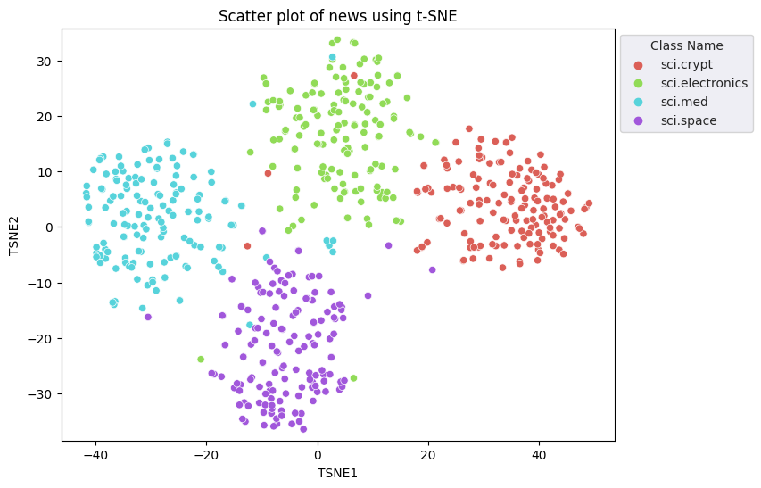
t 分散確率近傍エンベディング（t-SNE）アプローチを適用して、次元数を削減します。この手法では、次元の数を減らしながら、クラスタ（近接するポイント同士の距離を縮める）を維持できます。元のデータについて、他のデータポイントが「近傍」（意味が似ているなど）の分布を構築しようとします。次に、目的関数を最適化して、可視化において同様の分布を維持します。

tsne = TSNE(random_state=0, n_iter=1000)
tsne_results = tsne.fit_transform(X)

df_tsne = pd.DataFrame(tsne_results, columns=['TSNE1', 'TSNE2'])
df_tsne['Class Name'] = df_train['Class Name'] # Add labels column from df_train to df_tsne
df_tsne

fig, ax = plt.subplots(figsize=(8,6)) # Set figsize
sns.set_style('darkgrid', {"grid.color": ".6", "grid.linestyle": ":"})
sns.scatterplot(data=df_tsne, x='TSNE1', y='TSNE2', hue='Class Name', palette='hls')
sns.move_legend(ax, "upper left", bbox_to_anchor=(1, 1))
plt.title('Scatter plot of news using t-SNE');
plt.xlabel('TSNE1');
plt.ylabel('TSNE2');
plt.axis('equal')

(-46.191162300109866,
 53.521015357971194,
 -39.96646995544434,
 37.282975387573245)

png

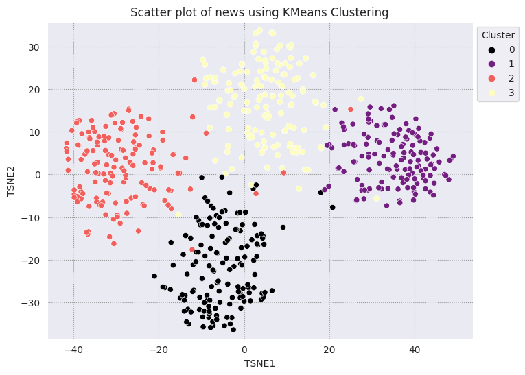
結果を K 平均法と比較する

K 平均法クラスタリングは一般的なクラスタリングアルゴリズムであり、教師なし学習によく使用されます。反復処理によって最適な k 個の中心点を決定し、各例を最も近い中心点に割り当てます。エンベディングを K 平均法アルゴリズムに直接入力し、エンベディングの可視化を ML アルゴリズムのパフォーマンスと比較する。

# Apply KMeans
kmeans_model = KMeans(n_clusters=4, random_state=1, n_init='auto').fit(X)
labels = kmeans_model.fit_predict(X)

df_tsne['Cluster'] = labels
df_tsne

fig, ax = plt.subplots(figsize=(8,6)) # Set figsize
sns.set_style('darkgrid', {"grid.color": ".6", "grid.linestyle": ":"})
sns.scatterplot(data=df_tsne, x='TSNE1', y='TSNE2', hue='Cluster', palette='magma')
sns.move_legend(ax, "upper left", bbox_to_anchor=(1, 1))
plt.title('Scatter plot of news using KMeans Clustering');
plt.xlabel('TSNE1');
plt.ylabel('TSNE2');
plt.axis('equal')

(-46.191162300109866,
 53.521015357971194,
 -39.96646995544434,
 37.282975387573245)

png

def get_majority_cluster_per_group(df_tsne_cluster, class_names):
  class_clusters = dict()
  for c in class_names:
    # Get rows of dataframe that are equal to c
    rows = df_tsne_cluster.loc[df_tsne_cluster['Class Name'] == c]
    # Get majority value in Cluster column of the rows selected
    cluster = rows.Cluster.mode().values[0]
    # Populate mapping dictionary
    class_clusters[c] = cluster
  return class_clusters

classes = df_tsne['Class Name'].unique()
class_clusters = get_majority_cluster_per_group(df_tsne, classes)
class_clusters

{'sci.crypt': 1, 'sci.electronics': 3, 'sci.med': 2, 'sci.space': 0}

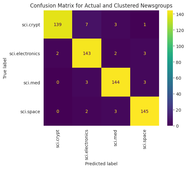
グループごとにクラスタの大半を取得し、そのクラスタ内にそのグループの実際のメンバーの数を確認する。

# Convert the Cluster column to use the class name
class_by_id = {v: k for k, v in class_clusters.items()}
df_tsne['Predicted'] = df_tsne['Cluster'].map(class_by_id.__getitem__)

# Filter to the correctly matched rows
correct = df_tsne[df_tsne['Class Name'] == df_tsne['Predicted']]

# Summarise, as a percentage
acc = correct['Class Name'].value_counts() / SAMPLE_SIZE
acc

sci.space          0.966667
sci.med            0.960000
sci.electronics    0.953333
sci.crypt          0.926667
Name: Class Name, dtype: float64

# Get predicted values by name
df_tsne['Predicted'] = ''
for idx, rows in df_tsne.iterrows():
  cluster = rows['Cluster']
  # Get key from mapping based on cluster value
  key = list(class_clusters.keys())[list(class_clusters.values()).index(cluster)]
  df_tsne.at[idx, 'Predicted'] = key

df_tsne

データに適用された K 平均法のパフォーマンスを可視化するには、混同行列を使用します。混同行列を使用すると、精度を超えて分類モデルのパフォーマンスを評価できます。誤って分類されたポイントがどのポイントに分類されるかを確認できます。ここには、上記の DataFrame で収集した実際の値と予測値が必要です。

cm = confusion_matrix(df_tsne['Class Name'].to_list(), df_tsne['Predicted'].to_list())
disp = ConfusionMatrixDisplay(confusion_matrix=cm,
                              display_labels=classes)
disp.plot(xticks_rotation='vertical')
plt.title('Confusion Matrix for Actual and Clustered Newsgroups');
plt.grid(False)

png

次のステップ

これで、クラスタリングを使用したエンベディングの可視化を独自に作成できました。独自のテキストデータを使用して、エンベディングとして可視化してみましょう。可視化のステップを完了するために、次元数を削減できます。TSNE は入力のクラスタリングは得意ですが、収束に時間がかかったり、局所的な最小値で行き詰まったりする可能性があるので注意してください。この問題が発生した場合は、主成分分析（PCA）という手法も検討できます。

KMeans 以外にも、密度ベースの空間クラスタリング（DBSCAN）など、他のクラスタリングアルゴリズムがあります。

エンベディングの使用方法について詳しくは、以下のチュートリアルをご覧ください。