前往 Gemma Cookbook 存放區取得產生與調整範例！瞭解詳情

本頁面由 Cloud Translation API 翻譯而成。

使用 Gemma 展示靈活的安全分類器

本程式碼研究室說明如何使用參數效率調整 (PET) 建立自訂文字分類器。PET 方法只會更新少量參數，而非微調整個模型，因此訓練起來相對容易且快速。這也讓模型能以相對較少的訓練資料學習新行為。Towards Agile Text Classifiers for Everyone一文詳細說明瞭這項方法，並說明如何將這些技術應用於各種安全性工作，只需幾百個訓練範例就能達到最先進的效能。

本程式碼研究室使用 LoRA PET 方法和較小的 Gemma 模型 (gemma_instruct_2b_en)，因為這樣執行速度和效率會更高。這個 Colab 涵蓋的步驟包括擷取資料、為 LLM 格式化資料、訓練 LoRA 權重，然後評估結果。這個程式碼研究室會以 ETHOS 資料集進行訓練，這是用於偵測仇恨言論的公開資料集，由 YouTube 和 Reddit 的留言所建構而成。當模型只以 200 個範例 (資料集的 1/4) 進行訓練時，F1 值為 0.80，ROC-AUC 值為 0.78，略高於排行榜上目前回報的 SOTA (截至本文撰寫時，即 2024 年 2 月 15 日)。在訓練完整的 800 個範例時，模型的 F1 分數為 83.74，ROC-AUC 分數為 88.17。較大的模型 (例如 gemma_instruct_7b_en) 通常效能較佳，但訓練和執行成本也會較高。

觸發警告：由於本程式碼研究室開發的安全分類器可偵測仇恨言論，因此範例和結果評估內容含有令人不快的字眼。

安裝和設定

在本程式碼研究室中，您需要最新版 keras (3)、keras-nlp (0.8.0) 和 Kaggle 帳戶，才能下載 Gemma 模型。

import kagglehub

kagglehub.login()

pip install -q -U keras-nlp
pip install -q -U keras

import os

os.environ["KERAS_BACKEND"] = "tensorflow"

載入 ETHOS 資料集

在本節中，您將載入資料集，以便訓練分類器，並將其預先處理為訓練和測試集。您將使用熱門研究資料集 ETHOS，該資料集是用於偵測社群媒體中的仇恨言論。如要進一步瞭解資料集的收集方式，請參閱論文「ETHOS：線上仇恨言論偵測資料集」。

import pandas as pd

gh_root = 'https://raw.githubusercontent.com'
gh_repo = 'intelligence-csd-auth-gr/Ethos-Hate-Speech-Dataset'
gh_path = 'master/ethos/ethos_data/Ethos_Dataset_Binary.csv'
data_url = f'{gh_root}/{gh_repo}/{gh_path}'

df = pd.read_csv(data_url, delimiter=';')
df['hateful'] = (df['isHate'] >= df['isHate'].median()).astype(int)

# Shuffle the dataset.
df = df.sample(frac=1, random_state=32)

# Split into train and test.
df_train, df_test = df[:800],  df[800:]

# Display a sample of the data.
df.head(5)[['hateful', 'comment']]

下載及例項化模型

如說明文件所述，您可以透過多種方式輕鬆使用 Gemma 模型。使用 Keras 時，您需要採取下列步驟：

import keras
import keras_nlp

# For reproducibility purposes.
keras.utils.set_random_seed(1234)

# Download the model from Kaggle using Keras.
model = keras_nlp.models.GemmaCausalLM.from_preset('gemma_instruct_2b_en')

# Set the sequence length to a small enough value to fit in memory in Colab.
model.preprocessor.sequence_length = 128

model.generate('Question: what is the capital of France? ', max_length=32)

文字預先處理和分隔符號符記

為了讓模型更瞭解我們的意圖，您可以對文字進行預處理，並使用分隔符權杖。這樣一來，模型就比較不會產生不符合預期格式的文字。舉例來說，您可以嘗試透過編寫類似以下的提示，向模型要求情緒分類：

Classify the following text into one of the following classes:[Positive,Negative]

Text: you look very nice today
Classification:

在這種情況下，模型可能會輸出您要的內容，也可能不會。舉例來說，如果文字含有換行字元，可能會對模型效能造成負面影響。更穩固的方法是使用分隔符權杖。提示會變成：

Classify the following text into one of the following classes:[Positive,Negative]
<separator>
Text: you look very nice today
<separator>
Prediction:

您可以使用預先處理文字的函式來抽象化這項作業：

def preprocess_text(
    text: str,
    labels: list[str],
    instructions: str,
    separator: str,
) -> str:
  prompt = f'{instructions}:[{",".join(labels)}]'
  return separator.join([prompt, f'Text:{text}', 'Prediction:'])

現在，如果您使用與先前相同的提示和文字執行函式，應該會得到相同的輸出內容：

text = 'you look very nice today'

prompt = preprocess_text(
    text=text,
    labels=['Positive', 'Negative'],
    instructions='Classify the following text into one of the following classes',
    separator='\n<separator>\n',
)

print(prompt)

Classify the following text into one of the following classes:[Positive,Negative]
<separator>
Text:you look very nice today
<separator>
Prediction:

輸出後置處理

模型的輸出內容是具有不同機率的符記。通常，您會從最可能的幾個符號中選取，並構建句子、段落，甚至是整份文件。不過，就分類而言，真正重要的是模型是否認為 Positive 比 Negative 更有可能，反之亦然。

假設您先前已將模型例項化，以下是如何將輸出內容處理成下一個符記分別為 Positive 或 Negative 的獨立機率：

import numpy as np


def compute_output_probability(
    model: keras_nlp.models.GemmaCausalLM,
    prompt: str,
    target_classes: list[str],
) -> dict[str, float]:
  # Shorthands.
  preprocessor = model.preprocessor
  tokenizer = preprocessor.tokenizer

  # NOTE: If a token is not found, it will be considered same as "<unk>".
  token_unk = tokenizer.token_to_id('<unk>')

  # Identify the token indices, which is the same as the ID for this tokenizer.
  token_ids = [tokenizer.token_to_id(word) for word in target_classes]

  # Throw an error if one of the classes maps to a token outside the vocabulary.
  if any(token_id == token_unk for token_id in token_ids):
    raise ValueError('One of the target classes is not in the vocabulary.')

  # Preprocess the prompt in a single batch. This is done one sample at a time
  # for illustration purposes, but it would be more efficient to batch prompts.
  preprocessed = model.preprocessor.generate_preprocess([prompt])

  # Identify output token offset.
  padding_mask = preprocessed["padding_mask"]
  token_offset = keras.ops.sum(padding_mask) - 1

  # Score outputs, extract only the next token's logits.
  vocab_logits = model.score(
      token_ids=preprocessed["token_ids"],
      padding_mask=padding_mask,
  )[0][token_offset]

  # Compute the relative probability of each of the requested tokens.
  token_logits = [vocab_logits[ix] for ix in token_ids]
  logits_tensor = keras.ops.convert_to_tensor(token_logits)
  probabilities = keras.activations.softmax(logits_tensor)

  return dict(zip(target_classes, probabilities.numpy()))

您可以使用先前建立的提示來執行該函式，以便測試該函式：

compute_output_probability(
    model=model,
    prompt=prompt,
    target_classes=['Positive', 'Negative'],
)

{'Positive': 0.99994016, 'Negative': 5.984089e-05}

將所有內容包裝為分類器

為了方便使用，您可以將所有剛建立的函式包裝成單一類似 sklearn 的分類器，並使用 predict() 和 predict_score() 等簡單易用且熟悉的函式。

import dataclasses


@dataclasses.dataclass(frozen=True)
class AgileClassifier:
  """Agile classifier to be wrapped around a LLM."""

  # The classes whose probability will be predicted.
  labels: tuple[str, ...]

  # Provide default instructions and control tokens, can be overridden by user.
  instructions: str = 'Classify the following text into one of the following classes'
  separator_token: str = '<separator>'
  end_of_text_token: str = '<eos>'

  def encode_for_prediction(self, x_text: str) -> str:
    return preprocess_text(
        text=x_text,
        labels=self.labels,
        instructions=self.instructions,
        separator=self.separator_token,
    )

  def encode_for_training(self, x_text: str, y: int) -> str:
    return ''.join([
        self.encode_for_prediction(x_text),
        self.labels[y],
        self.end_of_text_token,
    ])

  def predict_score(
      self,
      model: keras_nlp.models.GemmaCausalLM,
      x_text: str,
  ) -> list[float]:
    prompt = self.encode_for_prediction(x_text)
    token_probabilities = compute_output_probability(
        model=model,
        prompt=prompt,
        target_classes=self.labels,
    )
    return [token_probabilities[token] for token in self.labels]

  def predict(
      self,
      model: keras_nlp.models.GemmaCausalLM,
      x_eval: str,
  ) -> int:
    return np.argmax(self.predict_score(model, x_eval))

agile_classifier = AgileClassifier(labels=('Positive', 'Negative'))

模型微調

LoRA 是「Low-Rank Adaptation」的縮寫，這是一種微調技巧，可用來有效微調大型語言模型。如要進一步瞭解這項技術，請參閱 LoRA：大型語言模型的低秩調整論文。

Keras 實作的 Gemma 提供 enable_lora() 方法，可用於微調：

# Enable LoRA for the model and set the LoRA rank to 4.
model.backbone.enable_lora(rank=4)

啟用 LoRA 後，您就可以開始精細調整程序。在 Colab 上，每個 epoch 大約需要 5 分鐘：

import tensorflow as tf

# Create dataset with preprocessed text + labels.
map_fn = lambda x: agile_classifier.encode_for_training(*x)
x_train = list(map(map_fn, df_train[['comment', 'hateful']].values))
ds_train = tf.data.Dataset.from_tensor_slices(x_train).batch(2)

# Compile the model using the Adam optimizer and appropriate loss function.
model.compile(
    loss=keras.losses.SparseCategoricalCrossentropy(from_logits=True),
    optimizer=keras.optimizers.Adam(learning_rate=0.0005),
    weighted_metrics=[keras.metrics.SparseCategoricalAccuracy()],
)

# Begin training.
model.fit(ds_train, epochs=4)

Epoch 1/4
400/400 ━━━━━━━━━━━━━━━━━━━━ 354s 703ms/step - loss: 1.1365 - sparse_categorical_accuracy: 0.5874
Epoch 2/4
400/400 ━━━━━━━━━━━━━━━━━━━━ 338s 716ms/step - loss: 0.7579 - sparse_categorical_accuracy: 0.6662
Epoch 3/4
400/400 ━━━━━━━━━━━━━━━━━━━━ 324s 721ms/step - loss: 0.6818 - sparse_categorical_accuracy: 0.6894
Epoch 4/4
400/400 ━━━━━━━━━━━━━━━━━━━━ 323s 725ms/step - loss: 0.5922 - sparse_categorical_accuracy: 0.7220
<keras.src.callbacks.history.History at 0x7eb7e369c490>

訓練的週期越多，準確度就會越高，直到發生過度擬合為止。

檢查結果

您現在可以檢查剛訓練的敏捷分類器的輸出結果。這個程式碼會根據文字輸出預測類別分數：

text = 'you look really nice today'
scores = agile_classifier.predict_score(model, text)
dict(zip(agile_classifier.labels, scores))

{'Positive': 0.99899644, 'Negative': 0.0010035498}

Model Evaluation

最後，您將使用兩個常見指標來評估模型的效能，分別是 F1 分數和 AUC-ROC。F1 分數會在特定分類閾值下評估精確度與喚回度的調和平均數，以便找出偽陰性和偽陽性錯誤。另一方面，AUC-ROC 會在各種門檻中捕捉真陽率和偽陽率之間的取捨，並計算出這條曲線下的面積。

y_true = df_test['hateful'].values
# Compute the scores (aka probabilities) for each of the labels.
y_score = [agile_classifier.predict_score(model, x) for x in df_test['comment']]
# The label with highest score is considered the predicted class.
y_pred = np.argmax(y_score, axis=1)
# Extract the probability of a comment being considered hateful.
y_prob = [x[agile_classifier.labels.index('Negative')] for x in y_score]

from sklearn.metrics import f1_score, roc_auc_score

print(f'F1: {f1_score(y_true, y_pred):.2f}')
print(f'AUC-ROC: {roc_auc_score(y_true, y_prob):.2f}')

F1: 0.84
AUC-ROC: 0.88

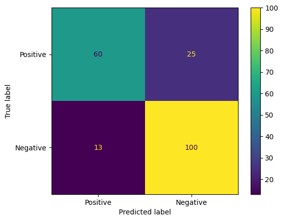
混淆矩陣是另一種評估模型預測結果的實用方法。混淆矩陣會以視覺化方式呈現不同類型的預測錯誤。

from sklearn.metrics import confusion_matrix, ConfusionMatrixDisplay

cm = confusion_matrix(y_true, y_pred)
ConfusionMatrixDisplay(
    confusion_matrix=cm,
    display_labels=agile_classifier.labels,
).plot()

<sklearn.metrics._plot.confusion_matrix.ConfusionMatrixDisplay at 0x7eb7e2d29ab0>

png

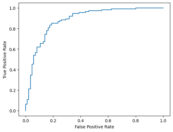
最後，您也可以查看 ROC 曲線，瞭解使用不同評分門檻時的潛在預測錯誤。

from sklearn.metrics import RocCurveDisplay, roc_curve

fpr, tpr, _ = roc_curve(y_true, y_prob, pos_label=1)
RocCurveDisplay(fpr=fpr, tpr=tpr).plot()

<sklearn.metrics._plot.roc_curve.RocCurveDisplay at 0x7eb4d130ef20>

png

附錄

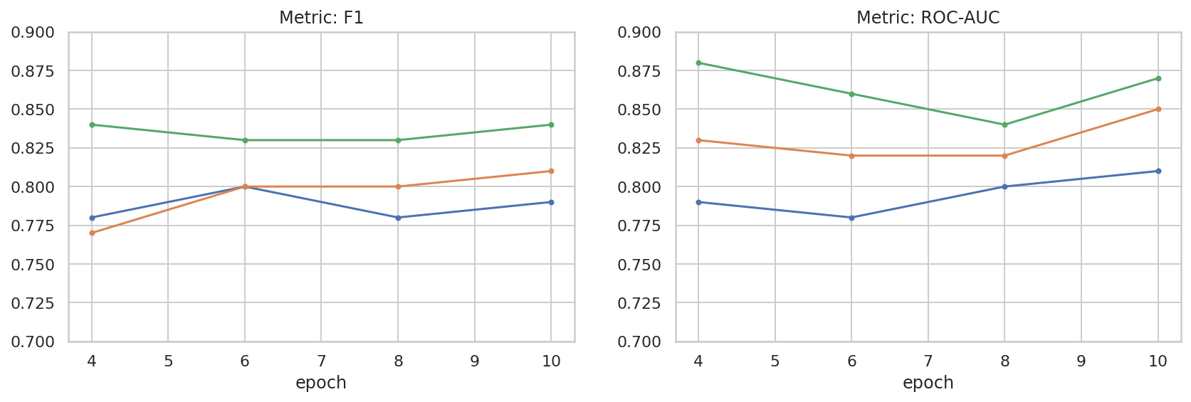
我們已對超參數空間進行一些基本探索，以便進一步瞭解資料集大小與成效之間的關係。請參閱下列圖表。

import matplotlib.pyplot as plt
import pandas as pd
import seaborn as sns

sns.set_theme(style="whitegrid")

results_f1 = pd.DataFrame([
    {'training_size': 800, 'epoch': 4, 'metric': 'f1', 'score': 0.84},
    {'training_size': 800, 'epoch': 6, 'metric': 'f1', 'score': 0.83},
    {'training_size': 800, 'epoch': 8, 'metric': 'f1', 'score': 0.83},
    {'training_size': 800, 'epoch': 10, 'metric': 'f1', 'score': 0.84},
    {'training_size': 400, 'epoch': 4, 'metric': 'f1', 'score': 0.77},
    {'training_size': 400, 'epoch': 6, 'metric': 'f1', 'score': 0.80},
    {'training_size': 400, 'epoch': 8, 'metric': 'f1', 'score': 0.80},
    {'training_size': 400, 'epoch': 10,'metric': 'f1', 'score': 0.81},
    {'training_size': 200, 'epoch': 4, 'metric': 'f1', 'score': 0.78},
    {'training_size': 200, 'epoch': 6, 'metric': 'f1', 'score': 0.80},
    {'training_size': 200, 'epoch': 8, 'metric': 'f1', 'score': 0.78},
    {'training_size': 200, 'epoch': 10, 'metric': 'f1', 'score': 0.79},
])

results_roc_auc = pd.DataFrame([
    {'training_size': 800, 'epoch': 4, 'metric': 'roc-auc', 'score': 0.88},
    {'training_size': 800, 'epoch': 6, 'metric': 'roc-auc', 'score': 0.86},
    {'training_size': 800, 'epoch': 8, 'metric': 'roc-auc', 'score': 0.84},
    {'training_size': 800, 'epoch': 10, 'metric': 'roc-auc', 'score': 0.87},
    {'training_size': 400, 'epoch': 4, 'metric': 'roc-auc', 'score': 0.83},
    {'training_size': 400, 'epoch': 6, 'metric': 'roc-auc', 'score': 0.82},
    {'training_size': 400, 'epoch': 8, 'metric': 'roc-auc', 'score': 0.82},
    {'training_size': 400, 'epoch': 10,'metric': 'roc-auc', 'score': 0.85},
    {'training_size': 200, 'epoch': 4, 'metric': 'roc-auc', 'score': 0.79},
    {'training_size': 200, 'epoch': 6, 'metric': 'roc-auc', 'score': 0.78},
    {'training_size': 200, 'epoch': 8, 'metric': 'roc-auc', 'score': 0.80},
    {'training_size': 200, 'epoch': 10, 'metric': 'roc-auc', 'score': 0.81},
])


plot_opts = dict(style='.-', ylim=(0.7, 0.9))
fig, (ax1, ax2) = plt.subplots(1, 2, figsize=(14, 4))
process_results_df = lambda df: df.set_index('epoch').groupby('training_size')['score']
process_results_df(results_f1).plot(title='Metric: F1', ax=ax1, **plot_opts)
process_results_df(results_roc_auc).plot(title='Metric: ROC-AUC', ax=ax2, **plot_opts)
fig.show()

png