|
|
|
 在 GitHub 上查看源代码 在 GitHub 上查看源代码
|
|
此 Codelab 展示了如何使用参数高效调优 (PET) 创建自定义文本分类器。PET 方法只会更新少量参数,而不是微调整个模型,因此训练起来相对容易且快速。这还可以让模型更轻松地利用相对较少的训练数据学习新行为。Towards Agile Text Classifiers for Everyone 详细介绍了该方法,其中展示了如何将这些技术应用于各种安全任务,并仅使用几百个训练示例即可实现最先进的性能。
此 Codelab 使用 LoRA PET 方法和较小的 Gemma 模型 (gemma_instruct_2b_en),因为该模型可以更快、更高效地运行。该 Colab 涵盖了提取数据、为 LLM 设置数据格式、训练 LoRA 权重,然后评估结果的步骤。此 Codelab 使用 ETHOS 数据集进行训练,该数据集是用于检测仇恨言论的公开数据集,由 YouTube 和 Reddit 评论构建而成。仅使用 200 个示例(数据集的 1/4)进行训练时,其 F1 得分为 0.80,ROC-AUC 得分为 0.78,略高于排行榜上目前报告的 SOTA(截至本文撰写之时,即 2024 年 2 月 15 日)。在使用完整的 800 个示例进行训练后,其 F1 得分为 83.74,ROC-AUC 得分为 88.17。较大的模型(例如 gemma_instruct_7b_en)通常效果更好,但训练和执行费用也更高。
触发警告:由于此 Codelab 开发了用于检测仇恨言论的安全分类器,因此示例和结果评估包含一些可怕的语言。
安装和设置
在本 Codelab 中,您需要使用较新版本的 keras (3) 和 keras-nlp (0.8.0),还需要一个 Kaggle 账号才能下载 Gemma 模型。
import kagglehub

kagglehub.login()
pip install -q -U keras-nlppip install -q -U keras
import os

os.environ["KERAS_BACKEND"] = "tensorflow"
加载 ETHOS 数据集
在本部分中,您将加载用于训练分类器的数据集,并将其预处理为训练集和测试集。您将使用热门研究数据集 ETHOS,该数据集旨在检测社交媒体中的仇恨言论。如需详细了解数据集的收集方式,请参阅ETHOS:在线仇恨言论检测数据集一文。
import pandas as pd

gh_root = 'https://raw.githubusercontent.com'
gh_repo = 'intelligence-csd-auth-gr/Ethos-Hate-Speech-Dataset'
gh_path = 'master/ethos/ethos_data/Ethos_Dataset_Binary.csv'
data_url = f'{gh_root}/{gh_repo}/{gh_path}'

df = pd.read_csv(data_url, delimiter=';')
df['hateful'] = (df['isHate'] >= df['isHate'].median()).astype(int)

# Shuffle the dataset.
df = df.sample(frac=1, random_state=32)

# Split into train and test.
df_train, df_test = df[:800],  df[800:]

# Display a sample of the data.
df.head(5)[['hateful', 'comment']]
下载并实例化模型
如文档中所述,您可以通过多种方式轻松使用 Gemma 模型。使用 Keras 时,您需要执行以下操作:
import keras
import keras_nlp

# For reproducibility purposes.
keras.utils.set_random_seed(1234)

# Download the model from Kaggle using Keras.
model = keras_nlp.models.GemmaCausalLM.from_preset('gemma_instruct_2b_en')

# Set the sequence length to a small enough value to fit in memory in Colab.
model.preprocessor.sequence_length = 128
model.generate('Question: what is the capital of France? ', max_length=32)
文本预处理和分隔符令牌
为了帮助模型更好地理解我们的意图,您可以对文本进行预处理并使用分隔符令牌。这样,模型就更不太可能生成不符合预期格式的文本。例如,您可以尝试编写如下提示,请求模型进行情感分类:
Classify the following text into one of the following classes:[Positive,Negative]

Text: you look very nice today
Classification:
在这种情况下,模型可能会输出您要找的内容,也可能不会。例如,如果文本包含换行符,则可能会对模型性能产生负面影响。更可靠的方法是使用分隔符令牌。然后,提示将变为:
Classify the following text into one of the following classes:[Positive,Negative]
<separator>
Text: you look very nice today
<separator>
Prediction:
可以使用预处理文本的函数对此进行抽象化处理:
def preprocess_text(
    text: str,
    labels: list[str],
    instructions: str,
    separator: str,
) -> str:
  prompt = f'{instructions}:[{",".join(labels)}]'
  return separator.join([prompt, f'Text:{text}', 'Prediction:'])
现在,如果您使用与之前相同的提示和文本运行该函数,应该会得到相同的输出:
text = 'you look very nice today'

prompt = preprocess_text(
    text=text,
    labels=['Positive', 'Negative'],
    instructions='Classify the following text into one of the following classes',
    separator='\n<separator>\n',
)

print(prompt)
Classify the following text into one of the following classes:[Positive,Negative]
<separator>
Text:you look very nice today
<separator>
Prediction:
输出后处理
模型的输出是具有不同概率的令牌。通常,为了生成文本,您需要从前几个概率最高的词元中进行选择,并构造句子、段落甚至完整的文档。不过,对于分类而言,真正重要的是模型认为 Positive 比 Negative 更有可能,还是 Negative 比 Positive 更有可能。
假设您之前实例化了模型,那么您可以按如下方式将其输出处理为下一个令牌分别为 Positive 或 Negative 的独立概率:
import numpy as np


def compute_output_probability(
    model: keras_nlp.models.GemmaCausalLM,
    prompt: str,
    target_classes: list[str],
) -> dict[str, float]:
  # Shorthands.
  preprocessor = model.preprocessor
  tokenizer = preprocessor.tokenizer

  # NOTE: If a token is not found, it will be considered same as "<unk>".
  token_unk = tokenizer.token_to_id('<unk>')

  # Identify the token indices, which is the same as the ID for this tokenizer.
  token_ids = [tokenizer.token_to_id(word) for word in target_classes]

  # Throw an error if one of the classes maps to a token outside the vocabulary.
  if any(token_id == token_unk for token_id in token_ids):
    raise ValueError('One of the target classes is not in the vocabulary.')

  # Preprocess the prompt in a single batch. This is done one sample at a time
  # for illustration purposes, but it would be more efficient to batch prompts.
  preprocessed = model.preprocessor.generate_preprocess([prompt])

  # Identify output token offset.
  padding_mask = preprocessed["padding_mask"]
  token_offset = keras.ops.sum(padding_mask) - 1

  # Score outputs, extract only the next token's logits.
  vocab_logits = model.score(
      token_ids=preprocessed["token_ids"],
      padding_mask=padding_mask,
  )[0][token_offset]

  # Compute the relative probability of each of the requested tokens.
  token_logits = [vocab_logits[ix] for ix in token_ids]
  logits_tensor = keras.ops.convert_to_tensor(token_logits)
  probabilities = keras.activations.softmax(logits_tensor)

  return dict(zip(target_classes, probabilities.numpy()))
您可以使用先前创建的提示运行该函数,以便对其进行测试:
compute_output_probability(
    model=model,
    prompt=prompt,
    target_classes=['Positive', 'Negative'],
)
{'Positive': 0.99994016, 'Negative': 5.984089e-05}
将所有内容封装为分类器
为方便使用,您可以将刚刚创建的所有函数封装到一个类似 sklearn 的分类器中,其中包含易于使用且熟悉的函数,例如 predict() 和 predict_score()。
import dataclasses


@dataclasses.dataclass(frozen=True)
class AgileClassifier:
  """Agile classifier to be wrapped around a LLM."""

  # The classes whose probability will be predicted.
  labels: tuple[str, ...]

  # Provide default instructions and control tokens, can be overridden by user.
  instructions: str = 'Classify the following text into one of the following classes'
  separator_token: str = '<separator>'
  end_of_text_token: str = '<eos>'

  def encode_for_prediction(self, x_text: str) -> str:
    return preprocess_text(
        text=x_text,
        labels=self.labels,
        instructions=self.instructions,
        separator=self.separator_token,
    )

  def encode_for_training(self, x_text: str, y: int) -> str:
    return ''.join([
        self.encode_for_prediction(x_text),
        self.labels[y],
        self.end_of_text_token,
    ])

  def predict_score(
      self,
      model: keras_nlp.models.GemmaCausalLM,
      x_text: str,
  ) -> list[float]:
    prompt = self.encode_for_prediction(x_text)
    token_probabilities = compute_output_probability(
        model=model,
        prompt=prompt,
        target_classes=self.labels,
    )
    return [token_probabilities[token] for token in self.labels]

  def predict(
      self,
      model: keras_nlp.models.GemmaCausalLM,
      x_eval: str,
  ) -> int:
    return np.argmax(self.predict_score(model, x_eval))

agile_classifier = AgileClassifier(labels=('Positive', 'Negative'))
模型微调
LoRA 是“低秩自适应”的缩写。这是一种微调技术,可用于高效微调大语言模型。如需了解详情,请参阅LoRA:大语言模型的低秩自适应论文。
Gemma 的 Keras 实现提供了一个 enable_lora() 方法,可用于微调:
# Enable LoRA for the model and set the LoRA rank to 4.
model.backbone.enable_lora(rank=4)
启用 LoRA 后,您可以开始微调流程。在 Colab 上,每个 epoch 大约需要 5 分钟:
import tensorflow as tf

# Create dataset with preprocessed text + labels.
map_fn = lambda x: agile_classifier.encode_for_training(*x)
x_train = list(map(map_fn, df_train[['comment', 'hateful']].values))
ds_train = tf.data.Dataset.from_tensor_slices(x_train).batch(2)

# Compile the model using the Adam optimizer and appropriate loss function.
model.compile(
    loss=keras.losses.SparseCategoricalCrossentropy(from_logits=True),
    optimizer=keras.optimizers.Adam(learning_rate=0.0005),
    weighted_metrics=[keras.metrics.SparseCategoricalAccuracy()],
)

# Begin training.
model.fit(ds_train, epochs=4)
Epoch 1/4
400/400 ━━━━━━━━━━━━━━━━━━━━ 354s 703ms/step - loss: 1.1365 - sparse_categorical_accuracy: 0.5874
Epoch 2/4
400/400 ━━━━━━━━━━━━━━━━━━━━ 338s 716ms/step - loss: 0.7579 - sparse_categorical_accuracy: 0.6662
Epoch 3/4
400/400 ━━━━━━━━━━━━━━━━━━━━ 324s 721ms/step - loss: 0.6818 - sparse_categorical_accuracy: 0.6894
Epoch 4/4
400/400 ━━━━━━━━━━━━━━━━━━━━ 323s 725ms/step - loss: 0.5922 - sparse_categorical_accuracy: 0.7220
<keras.src.callbacks.history.History at 0x7eb7e369c490>
训练的迭代次数越多,准确性就越高,直到发生过拟合为止。
检查结果
现在,您可以检查刚刚训练的敏捷分类器的输出。以下代码会针对一段文本输出预测的类得分:
text = 'you look really nice today'
scores = agile_classifier.predict_score(model, text)
dict(zip(agile_classifier.labels, scores))
{'Positive': 0.99899644, 'Negative': 0.0010035498}
模型评估
最后,您将使用两个常见指标(F1 得分和 AUC-ROC)评估模型的性能。F1 得分通过评估特定分类阈值下精确率和召回率的调和平均数来捕获假负例和假正例错误。另一方面,AUC-ROC 捕获各种阈值下真正例率与假正例率之间的权衡,并计算此曲线下的面积。
y_true = df_test['hateful'].values
# Compute the scores (aka probabilities) for each of the labels.
y_score = [agile_classifier.predict_score(model, x) for x in df_test['comment']]
# The label with highest score is considered the predicted class.
y_pred = np.argmax(y_score, axis=1)
# Extract the probability of a comment being considered hateful.
y_prob = [x[agile_classifier.labels.index('Negative')] for x in y_score]
from sklearn.metrics import f1_score, roc_auc_score

print(f'F1: {f1_score(y_true, y_pred):.2f}')
print(f'AUC-ROC: {roc_auc_score(y_true, y_prob):.2f}')
F1: 0.84
AUC-ROC: 0.88
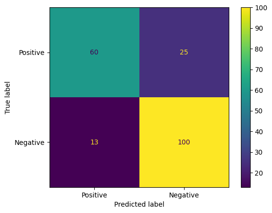
混淆矩阵是评估模型预测结果的另一种有趣方法。混淆矩阵会直观地描绘不同类型的预测错误。
from sklearn.metrics import confusion_matrix, ConfusionMatrixDisplay

cm = confusion_matrix(y_true, y_pred)
ConfusionMatrixDisplay(
    confusion_matrix=cm,
    display_labels=agile_classifier.labels,
).plot()
<sklearn.metrics._plot.confusion_matrix.ConfusionMatrixDisplay at 0x7eb7e2d29ab0>
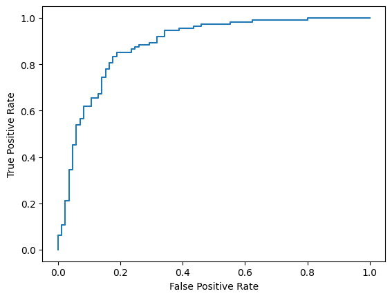
最后,您还可以查看 ROC 曲线,了解使用不同评分阈值时可能出现的预测错误。
from sklearn.metrics import RocCurveDisplay, roc_curve

fpr, tpr, _ = roc_curve(y_true, y_prob, pos_label=1)
RocCurveDisplay(fpr=fpr, tpr=tpr).plot()
<sklearn.metrics._plot.roc_curve.RocCurveDisplay at 0x7eb4d130ef20>
附录
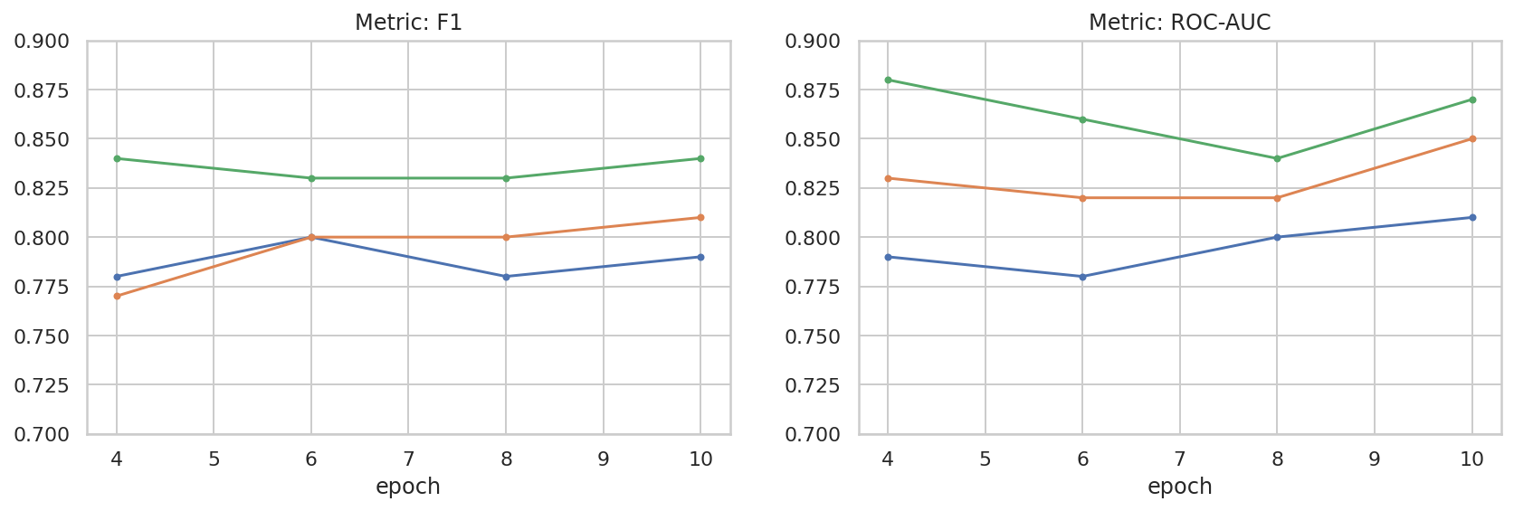
我们对超参数空间进行了一些基本探索,以便更好地了解数据集大小与性能之间的关系。请参阅以下图表。
import matplotlib.pyplot as plt
import pandas as pd
import seaborn as sns

sns.set_theme(style="whitegrid")

results_f1 = pd.DataFrame([
    {'training_size': 800, 'epoch': 4, 'metric': 'f1', 'score': 0.84},
    {'training_size': 800, 'epoch': 6, 'metric': 'f1', 'score': 0.83},
    {'training_size': 800, 'epoch': 8, 'metric': 'f1', 'score': 0.83},
    {'training_size': 800, 'epoch': 10, 'metric': 'f1', 'score': 0.84},
    {'training_size': 400, 'epoch': 4, 'metric': 'f1', 'score': 0.77},
    {'training_size': 400, 'epoch': 6, 'metric': 'f1', 'score': 0.80},
    {'training_size': 400, 'epoch': 8, 'metric': 'f1', 'score': 0.80},
    {'training_size': 400, 'epoch': 10,'metric': 'f1', 'score': 0.81},
    {'training_size': 200, 'epoch': 4, 'metric': 'f1', 'score': 0.78},
    {'training_size': 200, 'epoch': 6, 'metric': 'f1', 'score': 0.80},
    {'training_size': 200, 'epoch': 8, 'metric': 'f1', 'score': 0.78},
    {'training_size': 200, 'epoch': 10, 'metric': 'f1', 'score': 0.79},
])

results_roc_auc = pd.DataFrame([
    {'training_size': 800, 'epoch': 4, 'metric': 'roc-auc', 'score': 0.88},
    {'training_size': 800, 'epoch': 6, 'metric': 'roc-auc', 'score': 0.86},
    {'training_size': 800, 'epoch': 8, 'metric': 'roc-auc', 'score': 0.84},
    {'training_size': 800, 'epoch': 10, 'metric': 'roc-auc', 'score': 0.87},
    {'training_size': 400, 'epoch': 4, 'metric': 'roc-auc', 'score': 0.83},
    {'training_size': 400, 'epoch': 6, 'metric': 'roc-auc', 'score': 0.82},
    {'training_size': 400, 'epoch': 8, 'metric': 'roc-auc', 'score': 0.82},
    {'training_size': 400, 'epoch': 10,'metric': 'roc-auc', 'score': 0.85},
    {'training_size': 200, 'epoch': 4, 'metric': 'roc-auc', 'score': 0.79},
    {'training_size': 200, 'epoch': 6, 'metric': 'roc-auc', 'score': 0.78},
    {'training_size': 200, 'epoch': 8, 'metric': 'roc-auc', 'score': 0.80},
    {'training_size': 200, 'epoch': 10, 'metric': 'roc-auc', 'score': 0.81},
])


plot_opts = dict(style='.-', ylim=(0.7, 0.9))
fig, (ax1, ax2) = plt.subplots(1, 2, figsize=(14, 4))
process_results_df = lambda df: df.set_index('epoch').groupby('training_size')['score']
process_results_df(results_f1).plot(title='Metric: F1', ax=ax1, **plot_opts)
process_results_df(results_roc_auc).plot(title='Metric: ROC-AUC', ax=ax2, **plot_opts)
fig.show()