
|
|
|
 ดูแหล่งที่มาใน GitHub ดูแหล่งที่มาใน GitHub
|
ภาพรวม
ในสมุดบันทึกนี้ คุณจะได้เรียนรู้เกี่ยวกับการใช้การฝังที่ Gemini API สร้างขึ้นเพื่อฝึกโมเดลที่สามารถแยกประเภทโพสต์ของกลุ่มข่าวประเภทต่างๆ โดยอิงตามหัวข้อนั้นๆ
ในบทแนะนำนี้ คุณจะได้ฝึกตัวแยกประเภทให้คาดการณ์คลาสที่โพสต์ของกลุ่มข่าว
สิ่งที่ต้องดำเนินการก่อน
โดยคุณสามารถเรียกใช้การเริ่มต้นอย่างรวดเร็วนี้ใน Google Colab ได้
เพื่อให้การเริ่มต้นอย่างรวดเร็วนี้เสร็จสมบูรณ์ในสภาพแวดล้อมการพัฒนาของคุณเอง โปรดตรวจสอบว่าสภาพแวดล้อมของคุณเป็นไปตามข้อกำหนดต่อไปนี้
- Python 3.9 ขึ้นไป
- การติดตั้ง
jupyterเพื่อเรียกใช้สมุดบันทึก
ตั้งค่า
ก่อนอื่นให้ดาวน์โหลดและติดตั้งไลบรารี Gemini API Python
pip install -U -q google.generativeai
import re
import tqdm
import keras
import numpy as np
import pandas as pd

import google.generativeai as genai

# Used to securely store your API key
from google.colab import userdata

import seaborn as sns
import matplotlib.pyplot as plt

from keras import layers
from matplotlib.ticker import MaxNLocator
from sklearn.datasets import fetch_20newsgroups
import sklearn.metrics as skmetrics
รับคีย์ API
คุณต้องได้รับคีย์ API ก่อนจึงจะใช้ Gemini API ได้ หากยังไม่มี ให้สร้างคีย์ในคลิกเดียวใน Google AI Studio
ใน Colab ให้เพิ่มคีย์ไปยังเครื่องมือจัดการข้อมูลลับใต้ "🔑" ในแผงด้านซ้าย ตั้งชื่อว่า API_KEY
เมื่อมีคีย์ API แล้ว ให้ส่งคีย์ดังกล่าวไปยัง SDK โดยสามารถทำได้สองวิธี:
- ใส่คีย์ในตัวแปรสภาพแวดล้อม
GOOGLE_API_KEY(SDK จะดึงคีย์นั้นขึ้นมาโดยอัตโนมัติ) - ส่งคีย์ไปยัง
genai.configure(api_key=...)
# Or use `os.getenv('API_KEY')` to fetch an environment variable.
API_KEY=userdata.get('API_KEY')

genai.configure(api_key=API_KEY)
for m in genai.list_models():
  if 'embedContent' in m.supported_generation_methods:
    print(m.name)
models/embedding-001
models/embedding-001
ชุดข้อมูล
ชุดข้อมูลข้อความ 20 กลุ่มข่าวประกอบด้วยโพสต์ของกลุ่มข่าว 18,000 โพสต์ใน 20 หัวข้อที่แบ่งออกเป็นชุดการฝึกและการทดสอบ การแยกระหว่างชุดข้อมูลการฝึกและการทดสอบจะอิงตามข้อความที่โพสต์ก่อนและหลังวันที่ที่ระบุ สำหรับบทแนะนำนี้ คุณจะใช้ชุดข้อมูลย่อยของการฝึกและการทดสอบ คุณจะประมวลผลและจัดระเบียบข้อมูลล่วงหน้าลงใน Pandas DataFrame
newsgroups_train = fetch_20newsgroups(subset='train')
newsgroups_test = fetch_20newsgroups(subset='test')

# View list of class names for dataset
newsgroups_train.target_names
['alt.atheism',
 'comp.graphics',
 'comp.os.ms-windows.misc',
 'comp.sys.ibm.pc.hardware',
 'comp.sys.mac.hardware',
 'comp.windows.x',
 'misc.forsale',
 'rec.autos',
 'rec.motorcycles',
 'rec.sport.baseball',
 'rec.sport.hockey',
 'sci.crypt',
 'sci.electronics',
 'sci.med',
 'sci.space',
 'soc.religion.christian',
 'talk.politics.guns',
 'talk.politics.mideast',
 'talk.politics.misc',
 'talk.religion.misc']
ต่อไปนี้เป็นตัวอย่างลักษณะของจุดข้อมูลจากชุดการฝึก
idx = newsgroups_train.data[0].index('Lines')
print(newsgroups_train.data[0][idx:])
Lines: 15

 I was wondering if anyone out there could enlighten me on this car I saw
the other day. It was a 2-door sports car, looked to be from the late 60s/
early 70s. It was called a Bricklin. The doors were really small. In addition,
the front bumper was separate from the rest of the body. This is
all I know. If anyone can tellme a model name, engine specs, years
of production, where this car is made, history, or whatever info you
have on this funky looking car, please e-mail.

Thanks,

- IL
   ---- brought to you by your neighborhood Lerxst ----
ตอนนี้คุณจะเริ่มประมวลผลข้อมูลล่วงหน้าสำหรับบทแนะนำนี้ นำข้อมูลที่ละเอียดอ่อน เช่น ชื่อ อีเมล หรือส่วนที่ซ้ำซ้อนของข้อความออก เช่น "From: " และ "\nSubject: " จัดระเบียบข้อมูลลงใน Pandas DataFrame เพื่อให้อ่านได้ง่ายขึ้น
def preprocess_newsgroup_data(newsgroup_dataset):
  # Apply functions to remove names, emails, and extraneous words from data points in newsgroups.data
  newsgroup_dataset.data = [re.sub(r'[\w\.-]+@[\w\.-]+', '', d) for d in newsgroup_dataset.data] # Remove email
  newsgroup_dataset.data = [re.sub(r"\([^()]*\)", "", d) for d in newsgroup_dataset.data] # Remove names
  newsgroup_dataset.data = [d.replace("From: ", "") for d in newsgroup_dataset.data] # Remove "From: "
  newsgroup_dataset.data = [d.replace("\nSubject: ", "") for d in newsgroup_dataset.data] # Remove "\nSubject: "

  # Cut off each text entry after 5,000 characters
  newsgroup_dataset.data = [d[0:5000] if len(d) > 5000 else d for d in newsgroup_dataset.data]

  # Put data points into dataframe
  df_processed = pd.DataFrame(newsgroup_dataset.data, columns=['Text'])
  df_processed['Label'] = newsgroup_dataset.target
  # Match label to target name index
  df_processed['Class Name'] = ''
  for idx, row in df_processed.iterrows():
    df_processed.at[idx, 'Class Name'] = newsgroup_dataset.target_names[row['Label']]

  return df_processed
# Apply preprocessing function to training and test datasets
df_train = preprocess_newsgroup_data(newsgroups_train)
df_test = preprocess_newsgroup_data(newsgroups_test)

df_train.head()
ต่อไป คุณจะได้สุ่มตัวอย่างข้อมูลบางส่วนโดยนำจุดข้อมูล 100 จุดในชุดข้อมูลการฝึก แล้วตัดหมวดหมู่บางส่วนลงเพื่อดำเนินในบทแนะนำนี้ เลือกหมวดหมู่วิทยาศาสตร์เพื่อเปรียบเทียบ
def sample_data(df, num_samples, classes_to_keep):
  df = df.groupby('Label', as_index = False).apply(lambda x: x.sample(num_samples)).reset_index(drop=True)

  df = df[df['Class Name'].str.contains(classes_to_keep)]

  # Reset the encoding of the labels after sampling and dropping certain categories
  df['Class Name'] = df['Class Name'].astype('category')
  df['Encoded Label'] = df['Class Name'].cat.codes

  return df
TRAIN_NUM_SAMPLES = 100
TEST_NUM_SAMPLES = 25
CLASSES_TO_KEEP = 'sci' # Class name should contain 'sci' in it to keep science categories
df_train = sample_data(df_train, TRAIN_NUM_SAMPLES, CLASSES_TO_KEEP)
df_test = sample_data(df_test, TEST_NUM_SAMPLES, CLASSES_TO_KEEP)
df_train.value_counts('Class Name')
Class Name
sci.crypt          100
sci.electronics    100
sci.med            100
sci.space          100
dtype: int64
df_test.value_counts('Class Name')
Class Name
sci.crypt          25
sci.electronics    25
sci.med            25
sci.space          25
dtype: int64
สร้างการฝัง
ในส่วนนี้ คุณจะเห็นวิธีสร้างการฝังสำหรับข้อความโดยใช้การฝังจาก Gemini API หากต้องการดูข้อมูลเพิ่มเติมเกี่ยวกับการฝัง โปรดไปที่คู่มือการฝัง
การเปลี่ยนแปลง API เกี่ยวกับการฝังการฝัง-001
สำหรับโมเดลการฝังใหม่ จะมีพารามิเตอร์ประเภทงานใหม่และชื่อที่ไม่บังคับ (ใช้ได้กับ Tasks_type=RETRIEVAL_DOCUMENT เท่านั้น)
พารามิเตอร์ใหม่เหล่านี้จะใช้กับโมเดลการฝังใหม่ล่าสุดเท่านั้น ประเภทงานมีดังนี้
| ประเภทงาน | คำอธิบาย |
|---|---|
| RETRIEVAL_QUERY | ระบุว่าข้อความที่ระบุเป็นคำค้นหาในการตั้งค่าการค้นหา/ดึงข้อมูล |
| RETRIEVAL_DOCUMENT | ระบุว่าข้อความที่ระบุเป็นเอกสารในการตั้งค่าการค้นหา/ดึงข้อมูล |
| SEMANTIC_SIMILARITY | ระบุว่าจะใช้ข้อความที่กำหนดสำหรับความคล้ายคลึงกันของข้อความความหมาย (STS) |
| การจัดประเภท | ระบุว่าจะมีการใช้การฝังสำหรับการจัดประเภท |
| การคลัสเตอร์ | ระบุว่าจะมีการใช้การฝังสำหรับการจัดคลัสเตอร์ |
from tqdm.auto import tqdm
tqdm.pandas()

from google.api_core import retry

def make_embed_text_fn(model):

  @retry.Retry(timeout=300.0)
  def embed_fn(text: str) -> list[float]:
    # Set the task_type to CLASSIFICATION.
    embedding = genai.embed_content(model=model,
                                    content=text,
                                    task_type="classification")
    return embedding['embedding']

  return embed_fn

def create_embeddings(model, df):
  df['Embeddings'] = df['Text'].progress_apply(make_embed_text_fn(model))
  return df
model = 'models/embedding-001'
df_train = create_embeddings(model, df_train)
df_test = create_embeddings(model, df_test)
0%|          | 0/400 [00:00<?, ?it/s]
0%|          | 0/100 [00:00<?, ?it/s]
df_train.head()
สร้างโมเดลการจัดประเภทอย่างง่าย
ในที่นี้คุณจะกำหนดโมเดลง่ายๆ ที่มีเลเยอร์ที่ซ่อนอยู่หนึ่งเลเยอร์ และผลลัพธ์ความน่าจะเป็นของคลาสเดี่ยว การคาดคะเนจะสอดคล้องกับความน่าจะเป็นที่ข้อความหนึ่งๆ จะเป็นข่าวประเภทใดประเภทหนึ่ง เมื่อคุณสร้างโมเดล Keras จะสับเปลี่ยนจุดข้อมูลโดยอัตโนมัติ
def build_classification_model(input_size: int, num_classes: int) -> keras.Model:
  inputs = x = keras.Input(input_size)
  x = layers.Dense(input_size, activation='relu')(x)
  x = layers.Dense(num_classes, activation='sigmoid')(x)
  return keras.Model(inputs=[inputs], outputs=x)
# Derive the embedding size from the first training element.
embedding_size = len(df_train['Embeddings'].iloc[0])

# Give your model a different name, as you have already used the variable name 'model'
classifier = build_classification_model(embedding_size, len(df_train['Class Name'].unique()))
classifier.summary()

classifier.compile(loss = keras.losses.SparseCategoricalCrossentropy(from_logits=True),
                   optimizer = keras.optimizers.Adam(learning_rate=0.001),
                   metrics=['accuracy'])
Model: "model"
_________________________________________________________________
 Layer (type)                Output Shape              Param #
=================================================================
 input_1 (InputLayer)        [(None, 768)]             0

 dense (Dense)               (None, 768)               590592

 dense_1 (Dense)             (None, 4)                 3076

=================================================================
Total params: 593668 (2.26 MB)
Trainable params: 593668 (2.26 MB)
Non-trainable params: 0 (0.00 Byte)
_________________________________________________________________
embedding_size
768
ฝึกโมเดลเพื่อจำแนกกลุ่มข่าว
ขั้นตอนสุดท้าย คุณจะฝึกโมเดลง่ายๆ ได้ ใช้ Epoch จํานวนน้อยเพื่อหลีกเลี่ยงการปรับมากเกินไป Epoch แรกใช้เวลานานกว่าส่วนที่เหลือ เนื่องจากต้องคํานวณการฝังเพียงครั้งเดียว
NUM_EPOCHS = 20
BATCH_SIZE = 32

# Split the x and y components of the train and validation subsets.
y_train = df_train['Encoded Label']
x_train = np.stack(df_train['Embeddings'])
y_val = df_test['Encoded Label']
x_val = np.stack(df_test['Embeddings'])

# Train the model for the desired number of epochs.
callback = keras.callbacks.EarlyStopping(monitor='accuracy', patience=3)

history = classifier.fit(x=x_train,
                         y=y_train,
                         validation_data=(x_val, y_val),
                         callbacks=[callback],
                         batch_size=BATCH_SIZE,
                         epochs=NUM_EPOCHS,)
Epoch 1/20
/usr/local/lib/python3.10/dist-packages/keras/src/backend.py:5729: UserWarning: "`sparse_categorical_crossentropy` received `from_logits=True`, but the `output` argument was produced by a Softmax activation and thus does not represent logits. Was this intended?
  output, from_logits = _get_logits(
13/13 [==============================] - 1s 30ms/step - loss: 1.2141 - accuracy: 0.6675 - val_loss: 0.9801 - val_accuracy: 0.8800
Epoch 2/20
13/13 [==============================] - 0s 12ms/step - loss: 0.7580 - accuracy: 0.9400 - val_loss: 0.6061 - val_accuracy: 0.9300
Epoch 3/20
13/13 [==============================] - 0s 13ms/step - loss: 0.4249 - accuracy: 0.9525 - val_loss: 0.3902 - val_accuracy: 0.9200
Epoch 4/20
13/13 [==============================] - 0s 13ms/step - loss: 0.2561 - accuracy: 0.9625 - val_loss: 0.2597 - val_accuracy: 0.9400
Epoch 5/20
13/13 [==============================] - 0s 13ms/step - loss: 0.1693 - accuracy: 0.9700 - val_loss: 0.2145 - val_accuracy: 0.9300
Epoch 6/20
13/13 [==============================] - 0s 13ms/step - loss: 0.1240 - accuracy: 0.9850 - val_loss: 0.1801 - val_accuracy: 0.9600
Epoch 7/20
13/13 [==============================] - 0s 21ms/step - loss: 0.0931 - accuracy: 0.9875 - val_loss: 0.1623 - val_accuracy: 0.9400
Epoch 8/20
13/13 [==============================] - 0s 16ms/step - loss: 0.0736 - accuracy: 0.9925 - val_loss: 0.1418 - val_accuracy: 0.9600
Epoch 9/20
13/13 [==============================] - 0s 20ms/step - loss: 0.0613 - accuracy: 0.9925 - val_loss: 0.1315 - val_accuracy: 0.9700
Epoch 10/20
13/13 [==============================] - 0s 20ms/step - loss: 0.0479 - accuracy: 0.9975 - val_loss: 0.1235 - val_accuracy: 0.9600
Epoch 11/20
13/13 [==============================] - 0s 19ms/step - loss: 0.0399 - accuracy: 0.9975 - val_loss: 0.1219 - val_accuracy: 0.9700
Epoch 12/20
13/13 [==============================] - 0s 21ms/step - loss: 0.0326 - accuracy: 0.9975 - val_loss: 0.1158 - val_accuracy: 0.9700
Epoch 13/20
13/13 [==============================] - 0s 19ms/step - loss: 0.0263 - accuracy: 1.0000 - val_loss: 0.1127 - val_accuracy: 0.9700
Epoch 14/20
13/13 [==============================] - 0s 17ms/step - loss: 0.0229 - accuracy: 1.0000 - val_loss: 0.1123 - val_accuracy: 0.9700
Epoch 15/20
13/13 [==============================] - 0s 20ms/step - loss: 0.0195 - accuracy: 1.0000 - val_loss: 0.1063 - val_accuracy: 0.9700
Epoch 16/20
13/13 [==============================] - 0s 17ms/step - loss: 0.0172 - accuracy: 1.0000 - val_loss: 0.1070 - val_accuracy: 0.9700
ประเมินประสิทธิภาพของโมเดล
ใช้ Keras
Model.evaluate
เพื่อดูการสูญเสียและความแม่นยำของชุดข้อมูลทดสอบ
classifier.evaluate(x=x_val, y=y_val, return_dict=True)
4/4 [==============================] - 0s 4ms/step - loss: 0.1070 - accuracy: 0.9700
{'loss': 0.10700511932373047, 'accuracy': 0.9700000286102295}
วิธีหนึ่งในการประเมินประสิทธิภาพของโมเดลคือการแสดงภาพประสิทธิภาพของตัวแยกประเภท ใช้ plot_history เพื่อดูแนวโน้มการสูญเสียและความแม่นยำในช่วง Epoch
def plot_history(history):
  """
    Plotting training and validation learning curves.

    Args:
      history: model history with all the metric measures
  """
  fig, (ax1, ax2) = plt.subplots(1,2)
  fig.set_size_inches(20, 8)

  # Plot loss
  ax1.set_title('Loss')
  ax1.plot(history.history['loss'], label = 'train')
  ax1.plot(history.history['val_loss'], label = 'test')
  ax1.set_ylabel('Loss')

  ax1.set_xlabel('Epoch')
  ax1.legend(['Train', 'Validation'])

  # Plot accuracy
  ax2.set_title('Accuracy')
  ax2.plot(history.history['accuracy'],  label = 'train')
  ax2.plot(history.history['val_accuracy'], label = 'test')
  ax2.set_ylabel('Accuracy')
  ax2.set_xlabel('Epoch')
  ax2.legend(['Train', 'Validation'])

  plt.show()

plot_history(history)

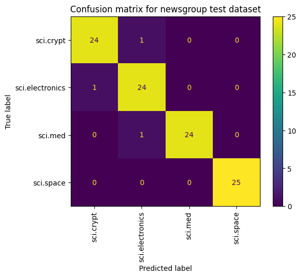
อีกวิธีหนึ่งในการดูประสิทธิภาพของโมเดลที่นอกเหนือจากการวัดการสูญเสียและความแม่นยำคือการใช้เมทริกซ์ความสับสน เมทริกซ์ความสับสนให้คุณประเมินประสิทธิภาพของโมเดลการจัดประเภทนอกเหนือจากความแม่นยำได้ คุณจะเห็นว่าคะแนนที่จัดประเภทไม่ถูกต้องรายการใดได้รับการจัดประเภท ในการสร้างเมทริกซ์ความสับสนสำหรับปัญหาการจัดประเภทแบบหลายคลาสนี้ ให้รับค่าจริงในชุดทดสอบและค่าที่คาดการณ์ไว้
เริ่มต้นด้วยการสร้างคลาสที่คาดการณ์สำหรับแต่ละตัวอย่างในชุดการตรวจสอบโดยใช้ Model.predict()
y_hat = classifier.predict(x=x_val)
y_hat = np.argmax(y_hat, axis=1)
4/4 [==============================] - 0s 4ms/step
labels_dict = dict(zip(df_test['Class Name'], df_test['Encoded Label']))
labels_dict
{'sci.crypt': 0, 'sci.electronics': 1, 'sci.med': 2, 'sci.space': 3}
cm = skmetrics.confusion_matrix(y_val, y_hat)
disp = skmetrics.ConfusionMatrixDisplay(confusion_matrix=cm,
                              display_labels=labels_dict.keys())
disp.plot(xticks_rotation='vertical')
plt.title('Confusion matrix for newsgroup test dataset');
plt.grid(False)
ขั้นตอนถัดไป
หากต้องการดูข้อมูลเพิ่มเติมเกี่ยวกับวิธีใช้การฝัง โปรดดูบทแนะนำอื่นๆ เหล่านี้